Savitzky-Golay derivatives on a synthetic spectrum

This example shows how to compute smoothed derivatives with the public differentiate() interface. The calculation is delegated to the Savitzky-Golay filter and illustrates the automatic coordinate-aware scaling introduced in SpectroChemPy 0.12.5.

The Savitzky-Golay algorithm assumes a uniformly spaced coordinate. When delta is omitted, the signed spacing is automatically detected from the coordinate. The resulting units follow the physical rule source_units / coordinate_units**derivative_order.

import spectrochempy as scp

Build a synthetic absorbance spectrum

We construct a smooth absorbance band on a wavenumber axis and add a small amount of noise so that the derivative is not trivially exact.

x = scp.Coord.linspace(500.0, 3500.0, 500, title="wavenumber")
x.units = "1/centimeter"

# Gaussian-like band centred at 2000 cm⁻¹
# (scp.gaussian uses FWHM; sigma = FWHM / (2*sqrt(2*ln2)))
sigma = 300.0
mu = 2000.0
fwhm = 2.35482 * sigma
y = scp.gaussian(x, ampl=1.0, pos=mu, width=fwhm, normalized=False)

# Add a small amount of deterministic Gaussian noise
noise = scp.normal(loc=0.0, scale=0.005, size=x.size, seed=42)
ds = scp.NDDataset(y.data + noise.data, units="absorbance")
ds.set_coordset(x=x)
ds.name = "synthetic band"

Smoothing

deriv=0 (the default) performs pure smoothing. A larger window removes more noise but may also distort sharp features.

ds_smooth = scp.savgol(ds, size=15, order=3, deriv=0)

ax = ds.plot(color="b", lw=1, label="noisy", figsize=(8, 4))
ax = ds_smooth.plot(clear=False, color="r", lw=2, label="smoothed")
ax.set_title("Savitzky-Golay smoothing (size=15, order=3)")
ax.set_xlabel("wavenumber / cm⁻¹")
ax.set_ylabel("absorbance")
_ = ax.legend(loc="best")

First derivative with automatic delta

derivative_order=1 triggers automatic detection of the signed spacing from the coordinate. The result carries the units absorbance / cm⁻¹, i.e. absorbance·cm.

ds_d1 = scp.differentiate(
    ds,
    derivative_order=1,
    size=15,
    polynomial_order=3,
)

# This is equivalent to scp.savgol(ds, size=15, order=3, deriv=1).

# The analytical derivative of a Gaussian is available for comparison:
# d/dx exp(-0.5*((x-mu)/sigma)^2) = -(x-mu)/sigma^2 * y
dy_dx = -(x.data - mu) / sigma**2 * y.data

# Plot the SG derivative and the analytical reference
ax = ds_d1.plot(color="r", lw=2, label="SG derivative", figsize=(8, 4))
ax.plot(x.data, dy_dx, color="b", ls="--", lw=1, label="analytical")
ax.set_title("First derivative (size=15, order=3)")
ax.set_xlabel("wavenumber / cm⁻¹")
ax.set_ylabel(f"derivative / ({ds_d1.units})")
_ = ax.legend(loc="best")

Descending coordinate

When the coordinate is stored in descending order (common for wavenumber data), the auto-detected delta is negative. The negative spacing compensates for the reversed sample order, so the derivative retains the correct physical dy/dx sign at a given wavenumber.

x_desc_data = x.data[::-1]
x_desc = scp.Coord(x_desc_data, title="wavenumber")
x_desc.units = "1/centimeter"
ds_desc = scp.NDDataset(y.data[::-1] + noise.data[::-1], units="absorbance")
ds_desc.set_coordset(x=x_desc)
ds_desc_d1 = scp.differentiate(
    ds_desc,
    derivative_order=1,
    size=15,
    polynomial_order=3,
)

ax = ds_desc_d1.plot(
    color="r", lw=2, label="SG derivative (descending)", figsize=(8, 4)
)
ax.plot(x_desc_data, dy_dx[::-1], color="b", ls="--", lw=1, label="analytical")
ax.set_title("First derivative on descending coordinate")
ax.set_xlabel("wavenumber / cm⁻¹")
ax.set_ylabel(f"derivative / ({ds_desc_d1.units})")
_ = ax.legend(loc="best")

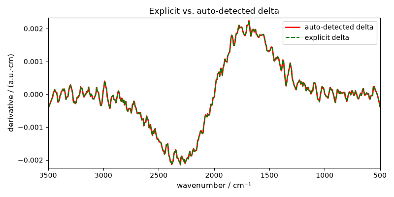
Explicit delta

An explicit delta disables auto-detection. The value is passed to SciPy with its sign and is interpreted in the unit of the coordinate. Here we supply the exact spacing (positive, because the coordinate is ascending) and obtain the same result as the automatic path.

delta = float(x.data[1] - x.data[0])
ds_d1_explicit = scp.differentiate(
    ds,
    derivative_order=1,
    size=15,
    polynomial_order=3,
    delta=delta,
)

# Plot the explicit-delta result on top of the auto-detected one
ax = ds_d1.plot(color="r", lw=2, label="auto-detected delta", figsize=(8, 4))
ax = ds_d1_explicit.plot(
    clear=False, color="g", ls="--", lw=1.5, label="explicit delta"
)
ax.set_title("Explicit vs. auto-detected delta")
ax.set_xlabel("wavenumber / cm⁻¹")
ax.set_ylabel(f"derivative / ({ds_d1.units})")
_ = ax.legend(loc="best")

Uncomment the following line to display all figures when running the script directly with Python.

# scp.show()