One-dimensional (1D) Fourier transformation
In this notebook, we are going to transform time-domain data into 1D or 2D spectra using SpectroChemPy processing tools
[1]:
import spectrochempy as scp

|
SpectroChemPy's API - v.0.7.0 © Copyright 2014-2025 - A.Travert & C.Fernandez @ LCS |
FFT of 1D NMR spectra
First we open read some time domain data. Here is a NMD free induction decay (FID):
[2]:
path = scp.preferences.datadir / "nmrdata" / "bruker" / "tests" / "nmr" / "topspin_1d"
fid = scp.read_topspin(path)
fid
[2]:
| name | topspin_1d expno:1 procno:1 (FID) |
| author | runner@fv-az1670-365 |
| created | 2025-02-18 09:42:42+00:00 |
| DATA | |
| title | intensity |
| values | R[ 1078 2284 ... 0.2342 -0.1008] pp I[ -1037 -2200 ... 0.06203 -0.05273] pp |
| size | 12411 (complex) |
| DIMENSION `x` | |
| size | 12411 |
| title | F1 acquisition time |
| coordinates | [ 0 4 ... 4.964e+04 4.964e+04] µs |
The type of the data is complex:
[3]:
fid.dtype
[3]:
dtype('complex128')
We can represent both real and imaginary parts on the same plot using the show_complex parameter.
[4]:
prefs = fid.preferences
prefs.figure.figsize = (6, 3)
_ = fid.plot(show_complex=True, xlim=(0, 15000))
print("td = ", fid.size)
td = 12411
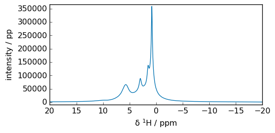
Now we perform a Fast Fourier Transform (FFT):
[5]:
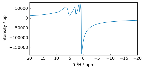
spec = scp.fft(fid)
_ = spec.plot(xlim=(100, -100))
print("si = ", spec.size)
spec
si = 16384
[5]:
| name | topspin_1d expno:1 procno:1 (FID) |
| author | runner@fv-az1670-365 |
| created | 2025-02-18 09:42:42+00:00 |
| history | 2025-02-18 09:42:43+00:00> `zf_size` shift performed on dimension `x` with parameters: {'size': 16384} 2025-02-18 09:42:43+00:00> Fft applied on dimension x 2025-02-18 09:42:43+00:00> Inplace binary op: imul with `[ 0.61+0.793j 0.61+0.793j ... 0.813+0.582j 0.813+0.582j]` 2025-02-18 09:42:43+00:00> `pk` applied to dimension `x` with parameters: {'phc0': 52.43836, 'phc1': -16.8366, 'pivot': 0.0, 'exptc': 0.0} |
| DATA | |
| title | intensity |
| values | R[ -1093 -1014 ... -1031 -1079] pp I[ -229.7 -126.8 ... 187.2 216.1] pp |
| size | 16384 (complex) |
| DIMENSION `x` | |
| size | 16384 |
| title | $\delta\ ^{1}H$ |
| coordinates | [ 253.1 253.1 ... -246.8 -246.8] ppm |
Alternative notation
[6]:
k = 1024
spec = fid.fft(size=32 * k)
_ = spec.plot(xlim=(100, -100))
print("si = ", spec.size)
si = 32768

[7]:
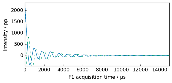
newfid = spec.ifft()
# x coordinate is in second (base units) so lets transform it
_ = newfid.plot(show_complex=True, xlim=(0, 15000))
Let’s compare fid and newfid. There differs as a rephasing has been automatically applied after the first FFT (with the parameters found in the original fid metadata: PHC0 and PHC1).
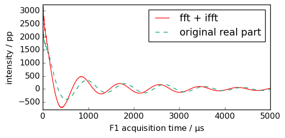
First point in the time domain of the real part is at the maximum.
[8]:
_ = newfid.real.plot(c="r", label="fft + ifft")
ax = fid.real.plot(clear=False, xlim=(0, 5000), ls="--", label="original real part")
_ = ax.legend()
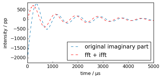
First point in the time domain of the imaginary part is at the minimum.
[9]:
_ = fid.imag.plot(ls="--", label="original imaginary part")
ax = newfid.imag.plot(clear=False, xlim=(0, 5000), c="r", label="fft + ifft")
_ = ax.legend(loc="lower right")
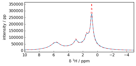
Preprocessing
Line broadening
Often before applying FFT, some exponential multiplication emor other broadening filters such as gm or sp are applied. See the dedicated apodization tutorial.
[10]:
fid2 = fid.em(lb="50. Hz")
spec2 = fid2.fft()
_ = spec2.plot()
_ = spec.plot(
    clear=False, xlim=(10, -5), c="r"
)  # superpose the non broadened spectrum in red and show expansion.
Zero-filling
[11]:
print("td = ", fid.size)
td = 12411
[12]:
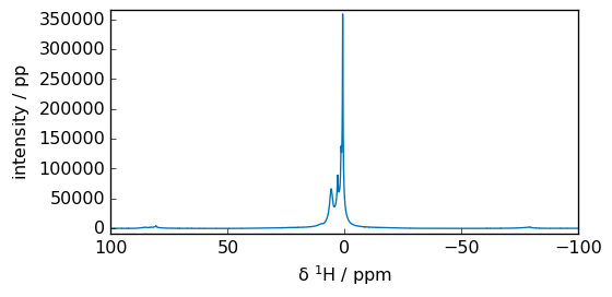
td = 64 * 1024  # size: 64 K
fid3 = fid.zf_size(size=td)
print("new td = ", fid3.x.size)
new td = 65536
[13]:
spec3 = fid3.fft()
_ = spec3.plot(xlim=(100, -100))
print("si = ", spec3.size)
si = 65536

Time domain baseline correction
See the dedicated Time domain baseline correction tutorial.
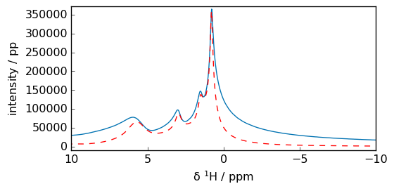
Magnitude calculation
[14]:
ms = spec.mc()
_ = ms.plot(xlim=(10, -10))
_ = spec.plot(clear=False, xlim=(10, -10), c="r")
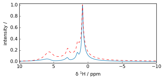
Power spectrum
[15]:
mp = spec.ps()
_ = (mp / mp.max()).plot()
_ = (spec / spec.max()).plot(
    clear=False, xlim=(10, -10), c="r"
)  # Here we have normalized the spectra at their max value.
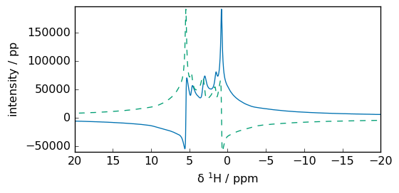
Real Fourier transform
In some case, it might be interesting to perform real Fourier transform . For instance, as a demonstration, we will independently transform real and imaginary part of the previous fid, and recombine them to obtain the same result as when performing complex fourier transform on the complex dataset.
[16]:
lim = (-20, 20)
_ = spec3.plot(xlim=lim)
_ = spec3.imag.plot(xlim=lim)

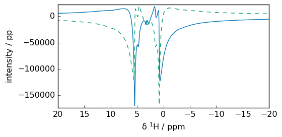
[17]:
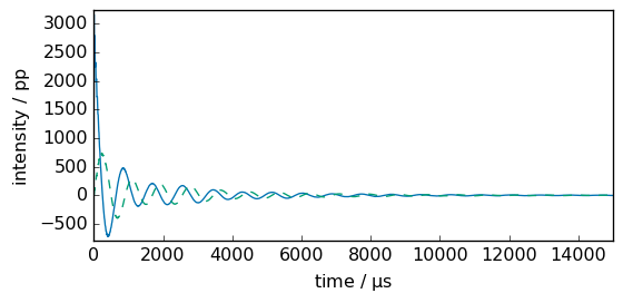
Re = fid3.real.astype("complex64")
fR = Re.fft()
_ = fR.plot(xlim=lim, show_complex=True)
Im = fid3.imag.astype("complex64")
fI = Im.fft()
_ = fI.plot(xlim=lim, show_complex=True)
Recombination:
[18]:
_ = (fR - fI.imag).plot(xlim=lim)
_ = (fR.imag + fI).plot(xlim=lim)