Advanced Matplotlib Integration

SpectroChemPy plots return Matplotlib Axes objects, giving you full access to Matplotlib’s capabilities.

Modifying the Axes

After plotting, customize using Matplotlib methods:

import spectrochempy as scp

ds = scp.read("irdata/nh4y-activation.spg")
ds1 = ds[0]

 WARNING | (UserWarning) Could not set locale: en_US or en_US.utf8

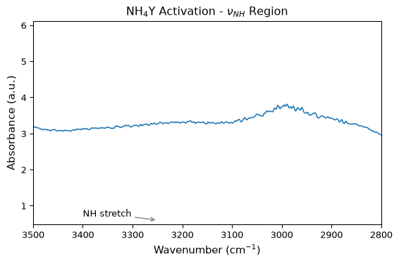
ax = ds1.plot()
_ = ax.set_title(r"NH$_4$Y Activation - $\nu_{NH}$ Region")
_ = ax.set_xlabel(r"Wavenumber (cm$^{-1}$)")
_ = ax.set_ylabel("Absorbance (a.u.)")
_ = ax.set_xlim(3500, 2800)
_ = ax.annotate(
    "NH stretch",
    xy=(3250, 0.6),
    xytext=(3400, 0.7),
    arrowprops={"arrowstyle": "->", "color": "gray"},
)

Multiple Plots

Create separate plots with different settings:

import matplotlib.pyplot as plt

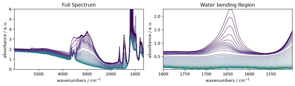
fig, (ax1, ax2) = plt.subplots(1, 2, figsize=(10, 3))

# Plot 1: full spectrum
_ = ds.plot(ax=ax1)
ax1.set_title("Full Spectrum")

# Plot 2: subset
_ = ds[:, 1800.0:1500.0].plot(ax=ax2)
ax2.set_title("Water bending Region")

plt.tight_layout()

Colormap Normalization

Advanced colormap normalization for special data scenarios:

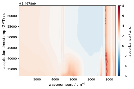
import matplotlib as mpl

# CenteredNorm - centers the colormap around a specific value
norm = mpl.colors.CenteredNorm(vcenter=1.0)
_ = ds.plot_image(cmap="RdBu_r", norm=norm, colorbar=True)

LaTeX-like Math in Labels

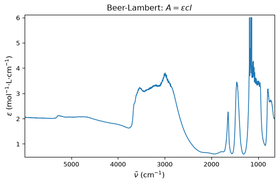
SpectroChemPy supports LaTeX math notation in labels:

ax = ds1.plot()
_ = ax.set_xlabel(r"$ \tilde{\nu}$ (cm$^{-1}$)")
_ = ax.set_ylabel(r"$ \epsilon$ (mol$^{-1}$·L·cm$^{-1}$)")
_ = ax.set_title(r"Beer-Lambert: $A = \epsilon c l$")

Saving Figures

The dataset plotting path and the figure-level helpers accept an output argument, which writes the finished figure to a file:

• ds.plot(output="spectrum.png"), for any method it dispatches

• the equivalent geometry shortcuts, such as ds.plot_pen(output="spectrum.png") or scp.plot_image(ds, output="map.png")

• scp.plot_multiple([ds, ds2], labels=["a", "b"], output="overlay.png")

• scp.multiplot([ds, ds2, ds3], output="grid.png")

• the analysis methods, such as pca.plot_score(), pca.plot_scree(), and pca.plot_merit(), plus analysis.plot_parity() where the model provides it

• the standalone composite functions, such as scp.plot_compare() and scp.plot_baseline()

The internal plot_1D(), plot_2D(), and plot_3D() renderers still only draw; public geometry shortcuts route through the shared lifecycle. The IRIS plugin keeps its own plotting methods, which are outside this contract.

The file name is used as given: the format follows the extension, and a name without extension is written with the savefig.format preference. Both str and pathlib.Path are accepted. Parent directories are never created silently - a missing directory is reported as an OSError.

The whole figure is written once the plot is complete, so legends, colorbars, titles, and multi-panel layouts are all part of the file. Saving happens before the display step, so combining output with show=True is safe.

from pathlib import Path
from tempfile import TemporaryDirectory

with TemporaryDirectory() as tmpdir:
    png_path = Path(tmpdir) / "spectrum.png"
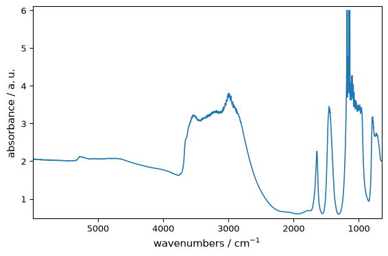
    _ = ds1.plot_pen(output=png_path, show=False)
    print(f"wrote {png_path.name}: {png_path.stat().st_size} bytes")

wrote spectrum.png: 104387 bytes

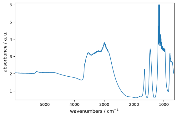
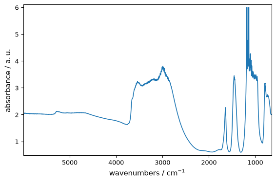
Matplotlib decides the file format from the extension, and vector formats stay vector:

with TemporaryDirectory() as tmpdir:
    _ = ds1.plot(output=Path(tmpdir) / "spectrum.svg", show=False)
    _ = ds1.plot(output=Path(tmpdir) / "spectrum.pdf", show=False)
    print(sorted(p.name for p in Path(tmpdir).iterdir()))

['spectrum.pdf', 'spectrum.svg']

The resolution, background, and bounding box of the written files come from the savefig preferences, so publication settings are changed once for the whole session:

prefs = scp.preferences
print("savefig dpi:", prefs.savefig_dpi)
print("savefig format:", prefs.savefig_format)
print("savefig transparent:", prefs.savefig_transparent)

savefig dpi: 300
savefig format: png
savefig transparent: False

prefs.savefig_dpi = 150
with TemporaryDirectory() as tmpdir:
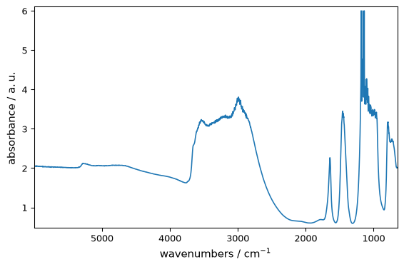
    _ = ds1.plot(output=Path(tmpdir) / "high_resolution.png", show=False)
prefs.savefig_dpi = 300  # restore the default

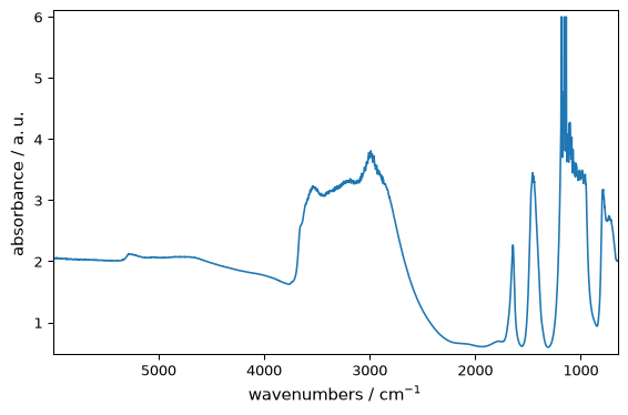
For anything the output argument does not cover, keep using Matplotlib directly on the returned axes or figure.

with TemporaryDirectory() as tmpdir:
    ax = ds1.plot(show=False)
    ax.figure.savefig(Path(tmpdir) / "manual.pdf", bbox_inches="tight")

Reproducibility

Avoid modifying global Matplotlib state. Instead:

• Use kwargs for per-plot settings

• Use preferences for session defaults

• Use styles for theme changes

Example of clean, reproducible plotting:

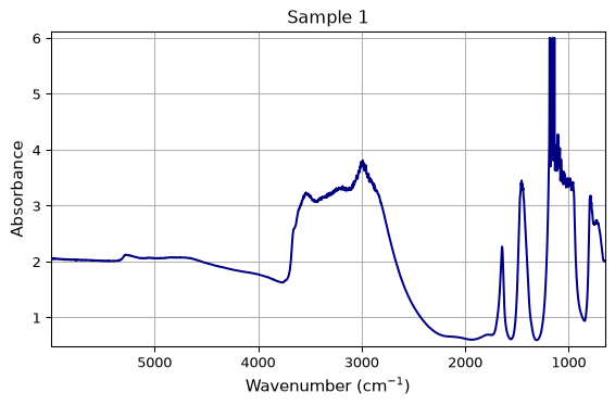
def plot_spectrum(dataset, title=None, output_path=None):
    """
    Plot a spectrum with consistent styling.

    The title and axis labels are passed to the plotting call itself, so that
    an ``output_path`` file contains the finished figure.
    """
    return dataset.plot(
        title=title,
        xlabel=r"Wavenumber (cm$^{-1}$)",
        ylabel="Absorbance",
        linewidth=1.5,
        color="navy",
        grid=True,
        output=output_path,
    )


# Each call produces consistent results
ax1 = plot_spectrum(ds1, title="Sample 1")
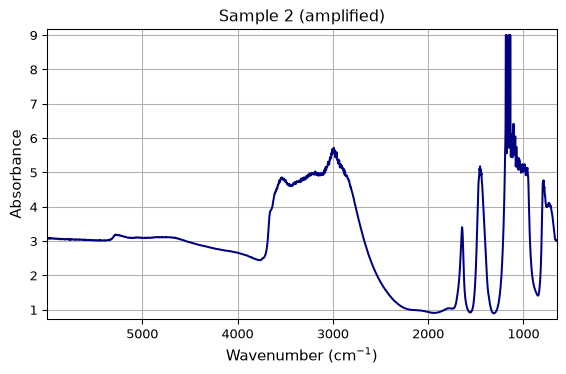
ax2 = plot_spectrum(ds1 * 1.5, title="Sample 2 (amplified)")

Where to Go Further

SpectroChemPy is built on Matplotlib. For advanced customization:

• Matplotlib Axes documentation

• Matplotlib customization guide

• SpectroChemPy API reference for plot method options

The combination of SpectroChemPy’s convenience with Matplotlib’s power gives you full control over your visualizations.