EFA example

In this example, we perform the Evolving Factor Analysis

import spectrochempy as scp

Load and preprocess the dataset

dataset = scp.read_omnic("irdata/nh4y-activation.spg")

Change the time origin

dataset.y -= dataset.y[0]

Mask saturated regions and preview

dataset[:, 1230.0:920.0] = scp.MASKED  # do not forget to use float in slicing
dataset[:, 5997.0:5993.0] = scp.MASKED

_ = dataset.plot_stack(title="NH4_Y activation dataset")

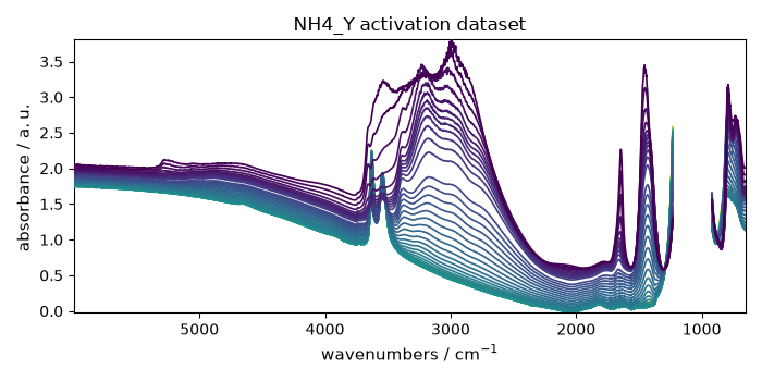
Fit the EFA model

efa1 = scp.EFA()
_ = efa1.fit(dataset)

Forward and backward evolution

Forward evolution of the first 5 components

f = efa1.f_ev[:, :5]
_ = f.T.plot(yscale="log", legend=f.k.labels)

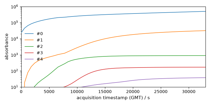
Note the use of coordinate k (component axis) in the expression above. To find the actual names of the coordinates, use the dims attribute:

f.dims

['y', 'k']

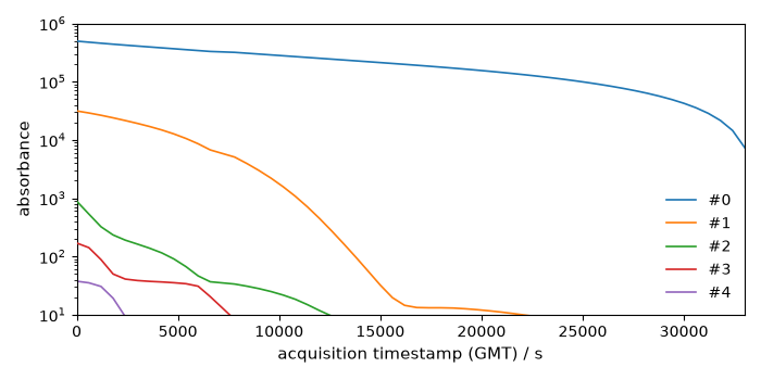
Backward evolution

b = efa1.b_ev[:, :5]
_ = b.T[:5].plot(yscale="log", legend=b.k.labels)

Select the number of components and extract concentrations

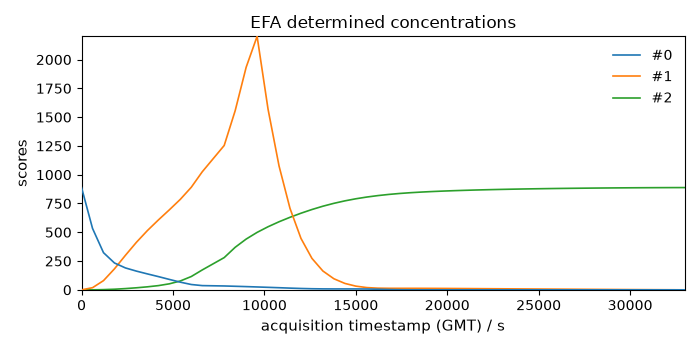
Use 3 components (the 4th component magnitude serves as the noise cutoff):

efa1.n_components = 3
efa1.cutoff = efa1.f_ev[:, 3].max()

C1 = efa1.transform()
_ = C1.T.plot(title="EFA determined concentrations", legend=C1.k.labels)

The same can be done in one step with fit_transform:

efa2 = scp.EFA(n_components=3)
C2 = efa2.fit_transform(dataset)
assert C1 == C2

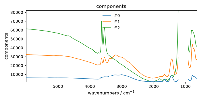
Extract the resolved components

St = efa2.get_components()
_ = St.plot(title="components", legend=St.k.labels)

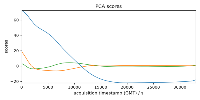
Compare with PCA

pca = scp.PCA(n_components=3)
C3 = pca.fit_transform(dataset)

_ = C3.T.plot(title="PCA scores")

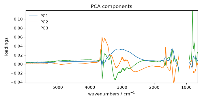
LT = pca.loadings
_ = LT.plot(title="PCA components", legend=LT.k.labels)

# Uncomment the following line to display all figures when running the script
# directly with Python.
#
# scp.show()