Solve a linear equation using LSTSQ

In this example, we find the least square solution of a simple linear equation.

# sphinx_gallery_thumbnail_number = 2

import spectrochempy as scp

Let’s take a similar example to the one given in the numpy.linalg documentation

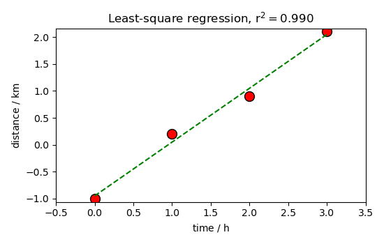
We have some noisy data that represent the distance d traveled by some objects versus time t:

t = scp.NDDataset(data=[0, 1, 2, 3], title="time", units="hour")

d = scp.NDDataset(
    data=[-1, 0.2, 0.9, 2.1], coordset=[t], title="distance", units="kilometer"
)

Here is a plot of these data-points:

d.plot_scatter(markersize=7, mfc="red")

<_Axes: xlabel='time $\\mathrm{/\\ \\mathrm{h}}$', ylabel='distance $\\mathrm{/\\ \\mathrm{km}}$'>

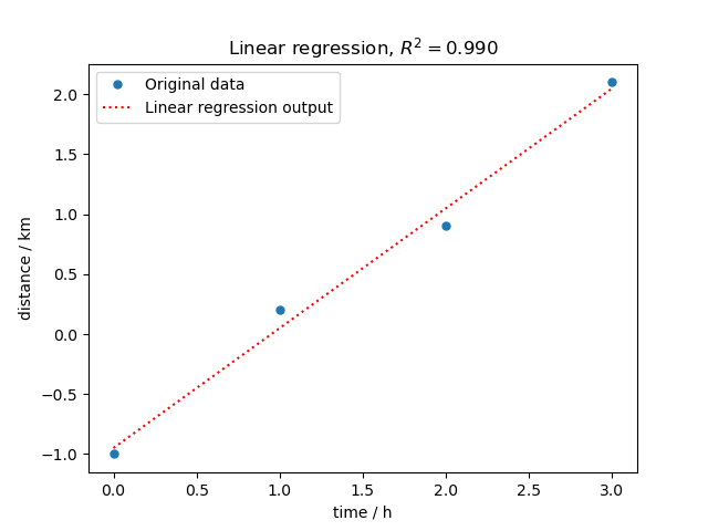
We want to fit a line through these data-points of equation

\[d = v.t + d_0\]

By examining the coefficients, we see that the line should have a gradient of roughly 1 km/h and cut the y-axis at, more or less, -1 km.

Using LSTSQ, the solution is found very easily:

lst = scp.LSTSQ(t, d)

v, d0 = lst.transform()
print("speed : {:.3fK},  d0 : {:.3fK}".format(v, d0))

speed : 1.000 kilometer.hour^-1,  d0 : -0.950 kilometer

Final plot

d.plot_scatter(
    markersize=10,
    mfc="red",
    mec="black",
    label="Original data",
    suptitle="Least-square fitting " "example",
)
dfit = lst.inverse_transform()

dfit.plot_pen(clear=False, color="g", label="Fitted line", legend=True)

<_Axes: xlabel='time $\\mathrm{/\\ \\mathrm{h}}$', ylabel='distance $\\mathrm{/\\ \\mathrm{km}}$'>

Note: The same result can be obtained directly using d as a single parameter on LSTSQ (as t is the x coordinate axis!)

lst = scp.LSTSQ(d)

v, d0 = lst.transform()
print("speed : {:.3fK},  d0 : {:.3fK}".format(v, d0))

# scp.show()  # uncomment to show plot if needed (not necessary in jupyter notebook)

speed : 1.000 kilometer.hour^-1,  d0 : -0.950 kilometer