Overview
The purpose of this page is to give you some quick examples of what can be done with SpectroChemPy.
See the gallery of examples and consult the user’s guide for more information on using SpectroChemPy
Before using the package, we must load the API (Application Programming Interface)
[1]:
import spectrochempy as scp

|
SpectroChemPy's API - v.0.6.8 © Copyright 2014-2024 - A.Travert & C.Fernandez @ LCS |
NDDataset, the main object
NDDataset is a python object, actually a container, which can represent most of your multidimensional spectroscopic data.
For instance, in the following we read data from a series of FTIR experiments, provided by the OMNIC software:
[2]:
ds = scp.read("irdata/nh4y-activation.spg")
Display dataset information
Short information:
[3]:
print(ds)
NDDataset: [float64] a.u. (shape: (y:55, x:5549))
Detailed information on the main metadata:
[4]:
ds
[4]:
| name | nh4y-activation |
| author | runner@fv-az1152-754 |
| created | 2024-03-08 01:01:24+00:00 |
| description | Omnic title: NH4Y-activation.SPG Omnic filename: /home/runner/.spectrochempy/testdata/irdata/nh4y-activation.spg |
| history | 2024-03-08 01:01:24+00:00> Imported from spg file /home/runner/.spectrochempy/testdata/irdata/nh4y-activation.spg. 2024-03-08 01:01:24+00:00> Sorted by date |
| DATA | |
| title | absorbance |
| values | [[ 2.057 2.061 ... 2.013 2.012] [ 2.033 2.037 ... 1.913 1.911] ... [ 1.794 1.791 ... 1.198 1.198] [ 1.816 1.815 ... 1.24 1.238]] a.u. |
| shape | (y:55, x:5549) |
| DIMENSION `x` | |
| size | 5549 |
| title | wavenumbers |
| coordinates | [ 6000 5999 ... 650.9 649.9] cm⁻¹ |
| DIMENSION `y` | |
| size | 55 |
| title | acquisition timestamp (GMT) |
| coordinates | [1.468e+09 1.468e+09 ... 1.468e+09 1.468e+09] s |
| labels | [[ 2016-07-06 19:03:14+00:00 2016-07-06 19:13:14+00:00 ... 2016-07-07 04:03:17+00:00 2016-07-07 04:13:17+00:00] [ vz0466.spa, Wed Jul 06 21:00:38 2016 (GMT+02:00) vz0467.spa, Wed Jul 06 21:10:38 2016 (GMT+02:00) ... vz0520.spa, Thu Jul 07 06:00:41 2016 (GMT+02:00) vz0521.spa, Thu Jul 07 06:10:41 2016 (GMT+02:00)]] |
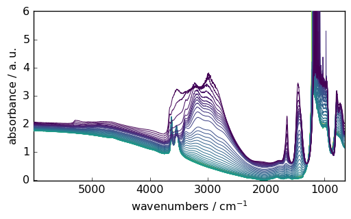
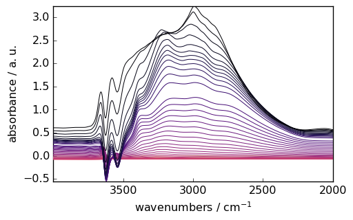
Plotting a dataset
[5]:
_ = ds.plot()
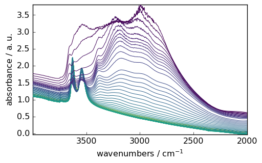
Slicing a dataset
[6]:
region = ds[:, 4000.0:2000.0]
_ = region.plot()
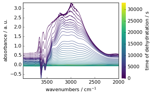
Maths on datasets
[7]:
region.y -= region.y[0]  # make y coordinate relative to the first point
region.y.title = "time of dehydratation"
region -= region[-1]  # suppress the last spectra to all
_ = region.plot(colorbar=True)
Processing a dataset
We just give here few examples
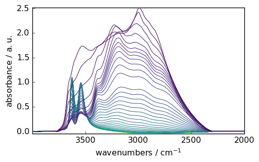
Smoothing
[8]:
smoothed = region.smooth(window_length=51, window="hanning")
_ = smoothed.plot(colormap="magma")
WARNING | (DeprecationWarning) The `window_length` attribute is now deprecated. Use `size` instead. `window_length` attribute will be removed in version 0.8.
Baseline correction
[9]:
region = ds[:, 4000.0:2000.0]
smoothed = region.smooth(window_length=51, window="hanning")
blc = scp.Baseline()
blc.ranges = [[2000.0, 2300.0], [3800.0, 3900.0]]
blc.multivariate = True
blc.model = "polynomial"
blc.order = "pchip"
blc.n_components = 5

_ = blc.fit(smoothed)
WARNING | (DeprecationWarning) The `window_length` attribute is now deprecated. Use `size` instead. `window_length` attribute will be removed in version 0.8.
[10]:
_ = blc.corrected.plot()
Analysis
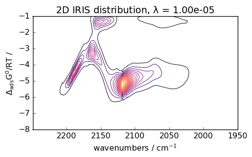
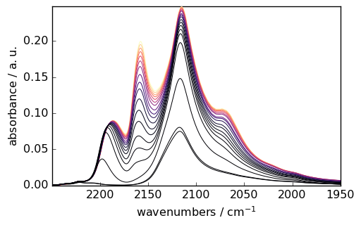
IRIS processing
[11]:
ds = scp.read_omnic("irdata/CO@Mo_Al2O3.SPG")[:, 2250.0:1950.0]
pressure = [
    0.00300,
    0.00400,
    0.00900,
    0.01400,
    0.02100,
    0.02600,
    0.03600,
    0.05100,
    0.09300,
    0.15000,
    0.20300,
    0.30000,
    0.40400,
    0.50300,
    0.60200,
    0.70200,
    0.80100,
    0.90500,
    1.00400,
]
ds.y = scp.Coord(pressure, title="Pressure", units="torr")
_ = ds.plot(colormap="magma")
[12]:
iris = scp.IRIS(reg_par=[-10, 1, 12])
K = scp.IrisKernel(ds, "langmuir", q=[-8, -1, 50])
iris.fit(ds, K)
_ = iris.plotdistribution(-7, colormap="magma")