PCA example (iris dataset)

In this example, we perform the PCA dimensionality reduction of the classical iris dataset (Ronald A. Fisher. “The Use of Multiple Measurements in Taxonomic Problems. Annals of Eugenics, 7, pp.179-188, 1936).

Load the SpectroChemPy API package

import spectrochempy as scp

Load the Iris dataset

dataset = scp.load_iris()

Fit a PCA model with automatic component selection

Using n_components="mle", the optimal number of components is determined automatically. Note: "mle" cannot be used when n_observations < n_features.

pca = scp.PCA(n_components="mle")
_ = pca.fit(dataset)

The number of components found is 3:

pca.n_components

3

It explains 99.5% of the variance:

pca.cumulative_explained_variance[-1].value

99.47878161267253 %

Fit a PCA model with a variance threshold

We can also specify the amount of explained variance directly:

pca = scp.PCA(n_components=0.999)
_ = pca.fit(dataset)

This time 4 components are found:

pca.n_components

4

Inspect the loadings and scores

The 4 components (loadings) are accessible via pca.components:

loadings = pca.components
loadings

NDDataset [`IRIS` Dataset_PCA.components] — float64, shape: (k:4, x:4)

name

:

`IRIS` Dataset_PCA.components

author

:

runner@runnervmzvulz

created

:

2026-08-16 03:09:08+00:00

description

:

components from PCA fit of `IRIS` Dataset.

history

:

2026-08-16 03:09:08+00:00> Created analysis output components with PCA from `IRIS` Dataset.

Data

title

:

components

values

:

[[ 0.3614 -0.08452 0.8567 0.3583]
[ 0.6566 0.7302 -0.1734 -0.07548]
[ -0.582 0.5979 0.07624 0.5458]
[ 0.3155 -0.3197 -0.4798 0.7537]]

shape

:

(k:4, x:4)

Dimension `k`

size

:

4

title

:

components

labels

:

[ PC1 PC2 PC3 PC4]

Dimension `x`

size

:

4

title

:

features

labels

:

[ sepal_length sepal width petal_length petal_width]

or equivalently via pca.loadings:

pca.loadings

NDDataset [`IRIS` Dataset_PCA.loadings] — float64, shape: (k:4, x:4)

name

:

`IRIS` Dataset_PCA.loadings

author

:

runner@runnervmzvulz

created

:

2026-08-16 03:09:08+00:00

description

:

loadings from PCA fit of `IRIS` Dataset.

history

:

2026-08-16 03:09:08+00:00> Created analysis output loadings with PCA from `IRIS` Dataset.

Data

title

:

loadings

values

:

[[ 0.3614 -0.08452 0.8567 0.3583]
[ 0.6566 0.7302 -0.1734 -0.07548]
[ -0.582 0.5979 0.07624 0.5458]
[ 0.3155 -0.3197 -0.4798 0.7537]]

shape

:

(k:4, x:4)

Dimension `k`

size

:

4

title

:

components

labels

:

[ PC1 PC2 PC3 PC4]

Dimension `x`

size

:

4

title

:

features

labels

:

[ sepal_length sepal width petal_length petal_width]

To reduce the data to a lower dimensionality, use transform:

scores = pca.transform()
scores

NDDataset [`IRIS` Dataset_PCA.scores] — float64, shape: (y:150, k:4)

name

:

`IRIS` Dataset_PCA.scores

author

:

runner@runnervmzvulz

created

:

2026-08-16 03:09:08+00:00

description

:

scores from PCA fit of `IRIS` Dataset.

history

:

2026-08-16 03:09:08+00:00> Created analysis output scores with PCA from `IRIS` Dataset.

Data

title

:

scores

values

:

[[ -2.684 0.3194 -0.02791 0.002262]
[ -2.714 -0.177 -0.2105 0.09903]
...
[ 1.901 0.1166 0.7233 0.0446]
[ 1.39 -0.2827 0.3629 -0.155]]

shape

:

(y:150, k:4)

Dimension `k`

size

:

4

title

:

components

labels

:

[ PC1 PC2 PC3 PC4]

Dimension `y`

size

:

150

title

:

samples

labels

:

[ setosa setosa ... virginica virginica]

The scores are also available directly via pca.scores:

scores = pca.scores
scores

NDDataset [`IRIS` Dataset_PCA.scores] — float64, shape: (y:150, k:4)

name

:

`IRIS` Dataset_PCA.scores

author

:

runner@runnervmzvulz

created

:

2026-08-16 03:09:08+00:00

description

:

scores from PCA fit of `IRIS` Dataset.

history

:

2026-08-16 03:09:08+00:00> Created analysis output scores with PCA from `IRIS` Dataset.

Data

title

:

scores

values

:

[[ -2.684 0.3194 -0.02791 0.002262]
[ -2.714 -0.177 -0.2105 0.09903]
...
[ 1.901 0.1166 0.7233 0.0446]
[ 1.39 -0.2827 0.3629 -0.155]]

shape

:

(y:150, k:4)

Dimension `k`

size

:

4

title

:

components

labels

:

[ PC1 PC2 PC3 PC4]

Dimension `y`

size

:

150

title

:

samples

labels

:

[ setosa setosa ... virginica virginica]

The explained and cumulative variance can be printed:

pca.printev()

Visualize the results

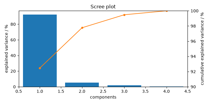
The scree plot shows the explained variance per component:

_ = pca.plot_scree()

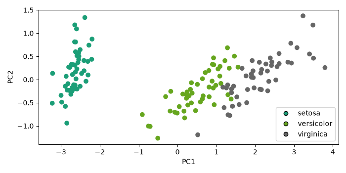
The 2D score plot (first 2 PCs) separates Iris-setosa from the other species:

_ = pca.plot_score(color_mapping="labels")

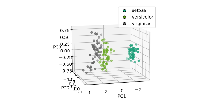
The 3D score plot (first 3 PCs) shows that a third PC does not further distinguish versicolor from virginica:

ax = pca.plot_score(components=(1, 2, 3), color_mapping="labels")
ax.view_init(10, 75)

This ends the example ! The following line can be uncommented if no plot shows when running the .py script with python

# scp.show()