NDDataset creation and plotting example

In this example, we create a 3D NDDataset from scratch, and then we plot one section (a 2D plane)

Creation

Now we will create a 3D NDDataset from scratch

import numpy as np

As usual, we start by loading the spectrochempy library

import spectrochempy as scp

Coordinates

The Coord object allows creating an array of coordinates directly with Coord.linspace, attaching metadata (units, labels, title) in a single step — no separate numpy array needed.

coord0 = scp.Coord.linspace(
    200.0,
    300.0,
    3,
    labels=["cold", "normal", "hot"],
    units="K",
    title="temperature",
)
coord1 = scp.Coord.linspace(0.0, 60.0, 100, units="minutes", title="time-on-stream")
coord2 = scp.Coord.linspace(4000.0, 1000.0, 100, units="cm^-1", title="wavenumber")

Labels can be useful for instance for indexing

a = coord0["normal"]
print(a)

Coord: [float64] K (size: 1)

Data and nd-Dataset

scp.fromfunction builds an NDDataset directly from a Python function. The function receives the coordinate arrays and returns the intensity values.

def synth_func(temperature, time, wavenumber):
    return np.sin(2.0 * np.pi * wavenumber / 4000.0) * np.exp(-time / 60) * temperature


mydataset = scp.fromfunction(
    synth_func,
    coordset=[coord0, coord1, coord2],
    title="Absorbance",
    units="absorbance",
)
mydataset.description = """Dataset example created for this tutorial.
It's a 3-D dataset (with dimensionless intensity: absorbance )"""
mydataset.name = "An example from scratch"
mydataset.author = "Blake and Mortimer"
print(mydataset)

NDDataset: [float64] a.u. (shape: (z:3, y:100, x:100))

We want to plot a section of this 3D NDDataset:

NDDataset can be sliced like conventional numpy-array…

new = mydataset[..., 0]

or maybe more conveniently in this case, using an axis labels:

new = mydataset["hot"]

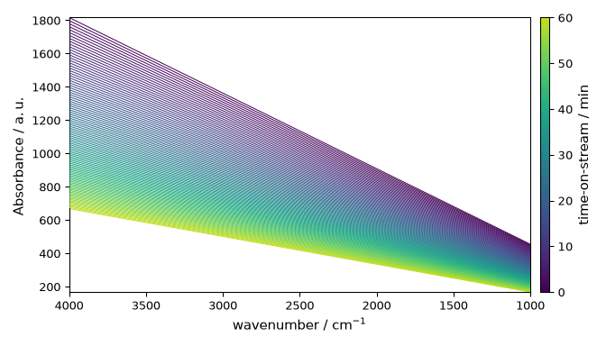
To plot a dataset, use the plot command (generic plot). As the section NDDataset is 2D, a stack plot is displayed by default. As you can see, the x-axis is in wavenumber and the ordinate axis is in absorbance units (au). The y dimension of the dataset is the time-on-stream (in minutes). Because the time-on-stream values are floats, this triggers the default sequential colormap (‘viridis’). The corresponding values can be seen if colorbar is passed as True:

_ = new.plot(colorbar=True)

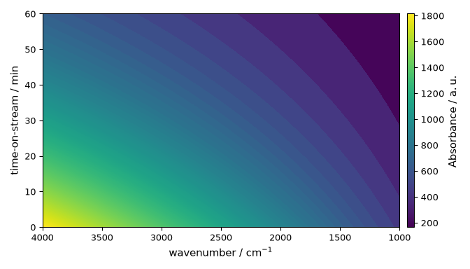
It is also possible to display this dataset as an image (actually a filled contour plot). The x is the same as before, but the ordinates are now the time-on-stream values. The color of the pixels is now related to the value of the absorbance. As the dataset contains both negative and positive values, the default colormap is diverging (RdBu).

sphinx_gallery_thumbnail_number = 2

_ = new.plot(method="image", colorbar=True)

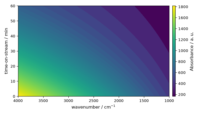
If a dataset contains only positive values, the default colormap is sequential (viridis):

_ = scp.abs(new).plot(method="image", colorbar=True)

_ = new.plot(method="map")
_ = scp.abs(new).plot(method="map")

• 
• 

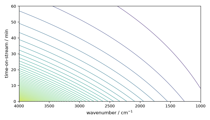
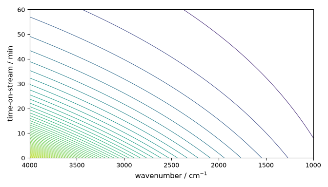
/home/runner/work/spectrochempy/tempdirs/scp_yf458zyp/src/spectrochempy/plotting/backends/matplotlib_backend.py:117: DeprecationWarning: The `method="map"` plotting alias is deprecated. Use `method="contour"` instead. It will not be removed before the SpectroChemPy deprecation policy is satisfied.
  method = normalize_backend_method(method, warned_aliases=_WARNED_ALIASES)

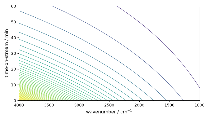
Note that the scp allows one to use this syntax too:

_ = scp.plot_map(new)

This ends the example ! The following line can be uncommented if no plot shows when running the .py script with python

# scp.show()