Exponential window multiplication

In this example, we perform exponential window multiplication to apodize a NMR signal in the time domain.

Requires the official spectrochempy-nmr plugin. Install with: pip install spectrochempy[nmr].

import spectrochempy as scp

Hz = scp.ur.Hz
us = scp.ur.us

path = scp.preferences.datadir / "nmrdata" / "bruker" / "tests" / "nmr" / "topspin_1d"
dataset1D = scp.nmr.read(path, expno=1, remove_digital_filter=True)

Normalize the dataset values and reduce the time domain

dataset1D /= dataset1D.real.data.max()  # normalize
dataset1D = dataset1D[0.0:15000.0]

Apply exponential window apodization

new1, curve1 = scp.em(dataset1D.copy(), lb=20 * Hz, retapod=True, inplace=False)

Apply a shifted exponential window apodization default units are HZ for broadening and microseconds for shifting

new2, curve2 = dataset1D.copy().em(
    lb=100 * Hz, shifted=10000 * us, retapod=True, inplace=False
)

Plotting

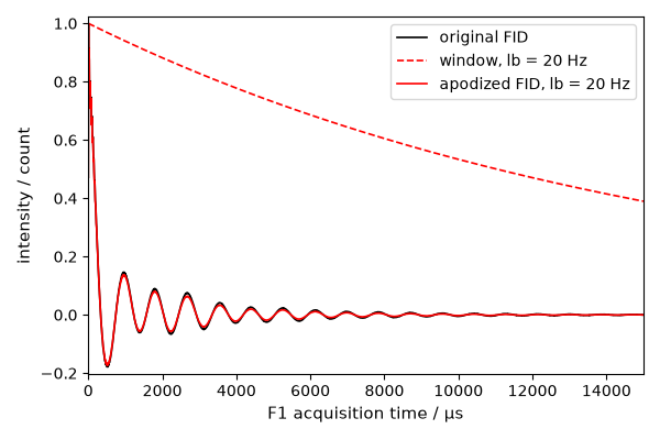
Compare the original FID with the exponential window and the apodized signal.

ax = dataset1D.real.plot(color="k", label="original FID", xlim=(0, 15000))
_ = curve1.plot(clear=False, color="r", ls="--", label="window, lb = 20 Hz")
_ = new1.real.plot(clear=False, color="r", label="apodized FID, lb = 20 Hz")
_ = ax.legend()

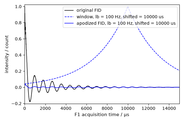
Shifted windows are easier to read on a separate figure.

ax = dataset1D.real.plot(color="k", label="original FID", xlim=(0, 15000))
_ = curve2.plot(
    clear=False,
    color="b",
    ls="--",
    label="window, lb = 100 Hz, shifted = 10000 us",
)
_ = new2.real.plot(
    clear=False,
    color="b",
    label="apodized FID, lb = 100 Hz, shifted = 10000 us",
)
_ = ax.legend()

This ends the example ! The following line can be uncommented if no plot shows when running the .py script with python scp.show()

sphinx_gallery_thumbnail_number = -1