Sine bell and squared Sine bell window multiplication

In this example, we use sine bell or squared sine bell window multiplication to apodize a NMR signal in the time domain.

Requires the official spectrochempy-nmr plugin. Install with: pip install spectrochempy[nmr].

import spectrochempy as scp

DATADIR = scp.preferences.datadir
path = DATADIR / "nmrdata" / "bruker" / "tests" / "nmr" / "topspin_1d"

dataset1D = scp.nmr.read(path, expno=1, remove_digital_filter=True)
dataset1D

NDDataset [topspin_1d expno:1 procno:1 (FID)] — complex128, size: 12411, count

name

:

topspin_1d expno:1 procno:1 (FID)

author

:

runner@runnervmzvulz

created

:

2026-08-16 03:08:08+00:00

history

:

2026-08-16 03:08:08+00:00> Imported from TopSpin dataset

Data

title

:

intensity

values

:

R[ 1078 2284 ... 0.2342 -0.1008] countI[ 1037 2200 ... -0.06203 0.05273] count

size

:

12411 (complex)

Dimension `x`

size

:

12411

title

:

F1 acquisition time

coordinates

:

[ 0 4 ... 4.964e+04 4.964e+04] µs

Normalize the dataset values and reduce the time domain

dataset1D /= dataset1D.real.data.max()  # normalize
dataset1D = dataset1D[0.0:15000.0]

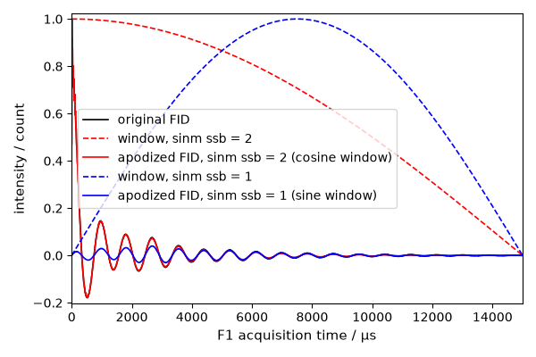
Apply Sine bell window apodization with parameter ssb=2, which correspond to a cosine function

new1, curve1 = scp.sinm(dataset1D, ssb=2, retapod=True, inplace=False)

this is equivalent to

new1, curve1 = dataset1D.sinm(ssb=2, retapod=True, inplace=False)

or also

new1, curve1 = scp.sp(dataset1D, ssb=2, pow=1, retapod=True, inplace=False)

Apply Sine bell window apodization with parameter ssb=2, which correspond to a sine function

new2, curve2 = dataset1D.sinm(ssb=1, retapod=True, inplace=False)

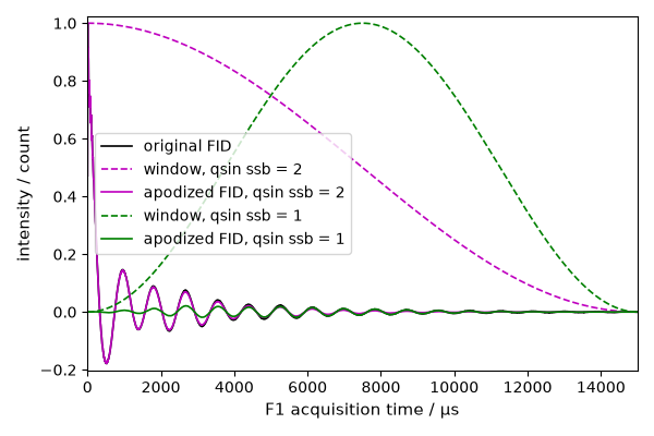
Apply Squared Sine bell window apodization with parameter ssb=1 and ssb=2

new3, curve3 = scp.qsin(dataset1D, ssb=2, retapod=True, inplace=False)
new4, curve4 = dataset1D.qsin(ssb=1, retapod=True, inplace=False)

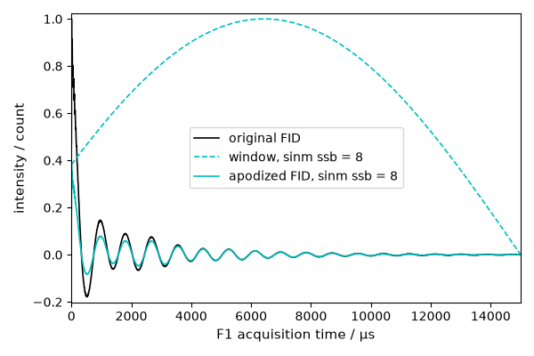
Apply shifted Sine bell window apodization with parameter ssb=8 (mixed sine/cosine window)

new5, curve5 = dataset1D.sinm(ssb=8, retapod=True, inplace=False)

Plotting

Compare sine bell windows on a first figure.

ax = dataset1D.real.plot(color="k", label="original FID", xlim=(0, 15000))
_ = curve1.plot(clear=False, color="r", ls="--", label="window, sinm ssb = 2")
_ = new1.real.plot(
    clear=False,
    color="r",
    label="apodized FID, sinm ssb = 2 (cosine window)",
)
_ = curve2.plot(clear=False, color="b", ls="--", label="window, sinm ssb = 1")
_ = new2.real.plot(
    clear=False,
    color="b",
    label="apodized FID, sinm ssb = 1 (sine window)",
)
_ = ax.legend()

Compare squared sine windows on a second figure.

ax = dataset1D.real.plot(color="k", label="original FID", xlim=(0, 15000))
_ = curve3.plot(clear=False, color="m", ls="--", label="window, qsin ssb = 2")
_ = new3.real.plot(clear=False, color="m", label="apodized FID, qsin ssb = 2")
_ = curve4.plot(clear=False, color="g", ls="--", label="window, qsin ssb = 1")
_ = new4.real.plot(clear=False, color="g", label="apodized FID, qsin ssb = 1")
_ = ax.legend()

Mixed sine/cosine windows are easier to inspect separately.

ax = dataset1D.real.plot(color="k", label="original FID", xlim=(0, 15000))
_ = curve5.plot(clear=False, color="c", ls="--", label="window, sinm ssb = 8")
_ = new5.real.plot(
    clear=False,
    color="c",
    label="apodized FID, sinm ssb = 8",
)
_ = ax.legend()

This ends the example ! The following line can be uncommented if no plot shows when running the .py script with python scp.show() sphinx_gallery_thumbnail_number = -1