NDDataset baseline correction

In this example, we perform a baseline correction of a 2D NDDataset interactively, using the multivariate method and a pchip/polynomial interpolation.

For comparison, we also use the asls`and `snip models.

Import the library

import spectrochempy as scp

Load and prepare the dataset

datadir = scp.preferences.datadir
nd = scp.read_omnic(datadir / "irdata" / "nh4y-activation.spg")

Keep only the spectral region of interest (use floats for coordinate-based slicing)

ndp = nd[:, 1291.0:5999.0]

Plot the raw dataset

_ = ndp.plot()

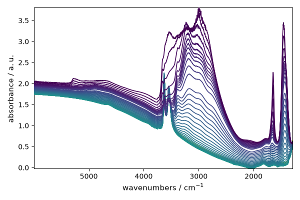
Quick linear baseline removal with basc:

ndp = ndp.basc()

Shift to positive values

offset = ndp.min()
ndp -= offset
_ = ndp.plot()

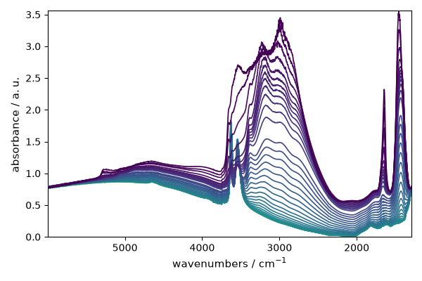
Multivariate baseline correction with pchip interpolation

Create a Baseline object using a multivariate approach with pchip (piecewise cubic Hermite) interpolation:

blc = scp.Baseline(
    log_level="WARNING",
    multivariate=True,
    model="polynomial",
    order="pchip",
    n_components=5,
)

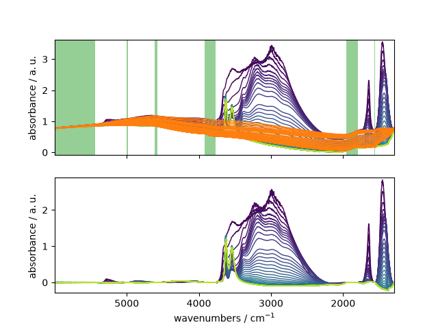
Define the reference regions for the baseline:

blc.ranges = [
    [1556.30, 1568.26],
    [1795.00, 1956.75],
    [3766.03, 3915.81],
    [4574.26, 4616.04],
    [4980.10, 4998.01],
    [5437.52, 5994.70],
]

Fit the model:

_ = blc.fit(ndp)

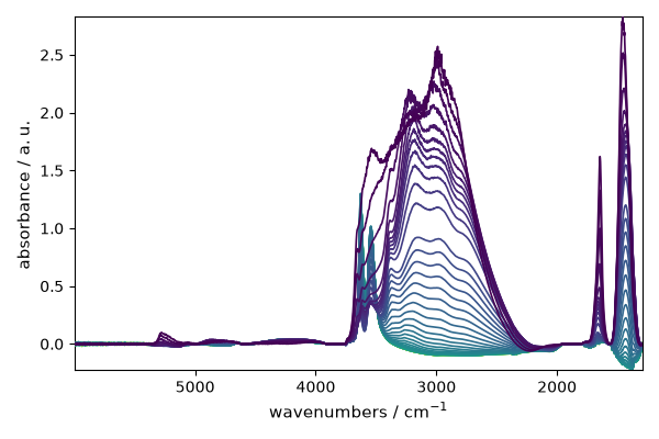
The baseline and corrected datasets are stored in the processor:

baseline = blc.baseline
corrected = blc.corrected

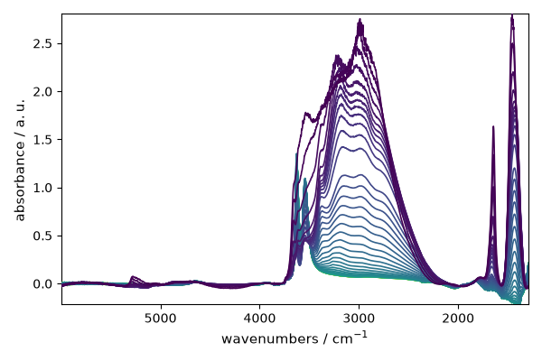
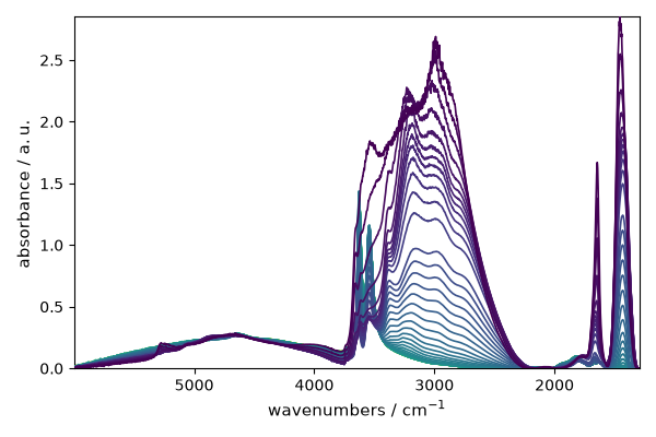
Plot the corrected dataset:

_ = corrected.plot()

A detailed view with region annotations:

ax = blc.plot(nb_traces=2, offset=50, show_regions=True)

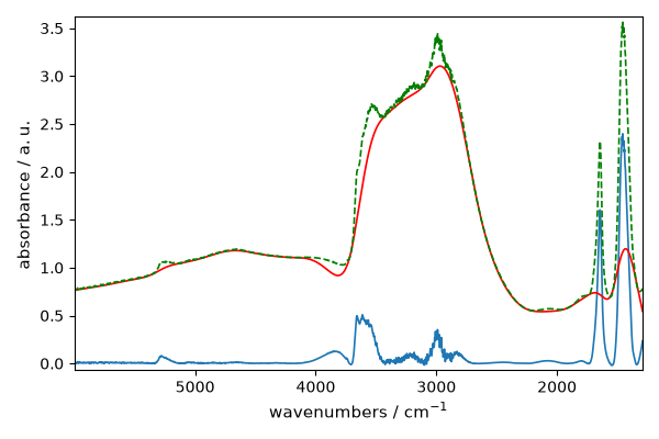
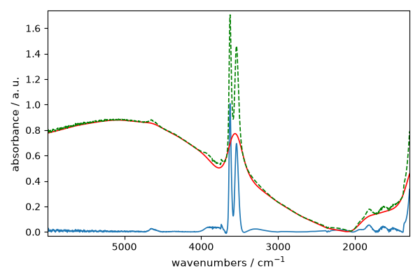
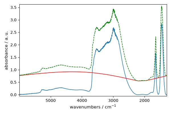
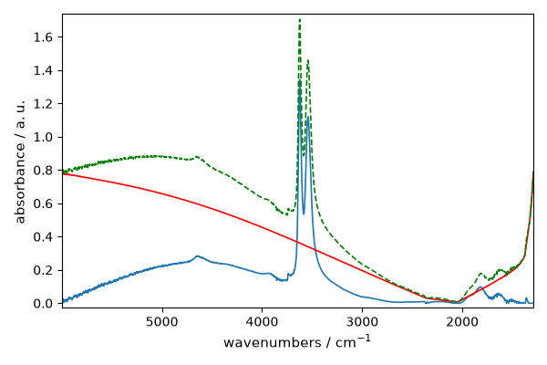
Compare individual spectra (corrected, baseline, original):

_ = corrected[0].plot()
_ = baseline[0].plot(clear=False, color="red", ls="-")
_ = ndp[0].plot(clear=False, color="green", ls="--")

_ = corrected[10].plot()
_ = baseline[10].plot(clear=False, color="red", ls="-")
_ = ndp[10].plot(clear=False, color="green", ls="--")

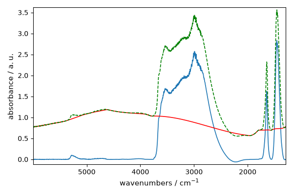
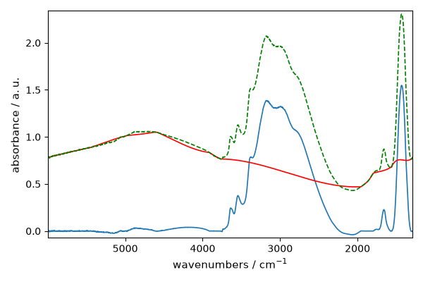
Switch to a polynomial model

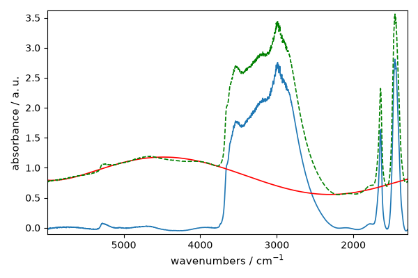
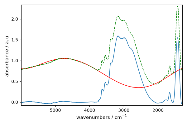
The pchip interpolation seems too rigid in some regions. We can change the model without redefining the Baseline object:

blc.model = "polynomial"
blc.order = 5

Refit and compare:

_ = blc.fit(ndp)

baseline = blc.baseline
corrected = blc.corrected

_ = corrected[0].plot()
_ = baseline[0].plot(clear=False, color="red", ls="-")
_ = ndp[0].plot(clear=False, color="green", ls="--")

_ = corrected[10].plot()
_ = baseline[10].plot(clear=False, color="red", ls="-")
_ = ndp[10].plot(clear=False, color="green", ls="--")

_ = corrected.plot()

Try the AsLS model

The Asymmetric Least Squares model (Eilers and Boelens, 2005) offers a different trade-off. The mu parameter controls smoothness and asymmetry controls the weighting.

blc.multivariate = False
blc.model = "asls"
blc.mu = 10**9
blc.asymmetry = 0.002
_ = blc.fit(ndp)

/home/runner/work/spectrochempy/tempdirs/scp_yf458zyp/src/spectrochempy/processing/baselineprocessing/baselineprocessing.py:527: SparseEfficiencyWarning: spsolve requires A be CSC or CSR matrix format
  z = spsolve(C, w * y)

baseline = blc.baseline
corrected = blc.corrected

_ = corrected[0].plot()
_ = baseline[0].plot(clear=False, color="red", ls="-")
_ = ndp[0].plot(clear=False, color="green", ls="--")

_ = corrected[-1].plot()
_ = baseline[-1].plot(clear=False, color="red", ls="-")
_ = ndp[-1].plot(clear=False, color="green", ls="--")

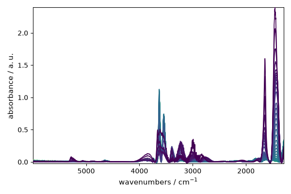
_ = corrected.plot()

Try the SNIP model

The Statistics-sensitive Non-linear Iterative Peak-clipping method:

blc.multivariate = False
blc.model = "snip"
blc.snip_width = 200
_ = blc.fit(ndp)

baseline = blc.baseline
corrected = blc.corrected

_ = corrected[0].plot()
_ = baseline[0].plot(clear=False, color="red", ls="-")
_ = ndp[0].plot(clear=False, color="green", ls="--")

_ = corrected[-1].plot()
_ = baseline[-1].plot(clear=False, color="red", ls="-")
_ = ndp[-1].plot(clear=False, color="green", ls="--")

_ = corrected.plot()

This ends the example ! The following line can be uncommented if no plot shows when running the .py script with python

# scp.show()