Note
Go to the end to download the full example code
Processing a 1D NMR spectrum
Basic 1D NMR processing and inspection with the official
spectrochempy-nmr plugin.
This example stays within the currently validated public scope of the plugin:
reading a 1D NMR dataset;
processing the FID to a frequency-domain spectrum with explicit SpectroChemPy parameters;
inspecting slices, correcting the baseline and picking peaks.
It does not claim replay of vendor processing parameters from metadata.
Import API
import numpy as np

import spectrochempy as scp
Import a 1D NMR FID
datadir = scp.preferences.datadir
nmrdir = datadir / "nmrdata"

fid = scp.nmr.read(nmrdir / "bruker" / "tests" / "nmr" / "topspin_1d" / "1" / "fid")
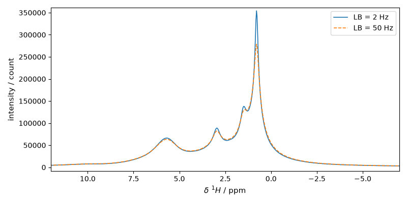
Compare two explicit apodization choices
The source FID is left unchanged. Each processed spectrum comes from its own
independent copy so the comparison is purely about the explicit lb value.
low_lb = scp.nmr.Experiment(fid.copy()).process(
    apodization="em",
    lb=2.0,
    size=16384,
    phase=None,
)
high_lb = scp.nmr.Experiment(fid.copy()).process(
    apodization="em",
    lb=50.0,
    size=16384,
    phase=None,
)
Overlay the two processed spectra on the same axes
ax = low_lb.plot(color="C0", label="LB = 2 Hz")
high_lb.plot(
    ax=ax,
    color="C1",
    linestyle="--",
    label="LB = 50 Hz",
    xlim=(-7.0, 12.0),
)
_ = ax.legend()
Continue with the mildly broadened spectrum
The rest of the example uses low_lb, which keeps the resolved multiplets
visually useful for peak picking and fitting.
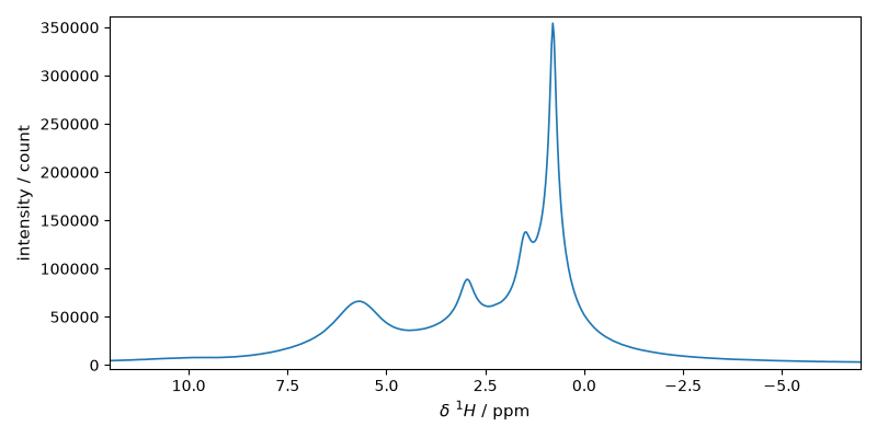
Select a region of interest
spectrum = dataset[-7.0:12.0]
_ = spectrum.plot()
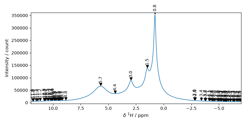
Peak picking
The ppm slice remains scientifically regular, but the current core Coord
machinery can still lose the linear flag after slicing because of
floating-point rounding on the sub-axis. Until that core behavior is fixed,
use plain point spacing for peak picking in this example so it remains fully
executable.
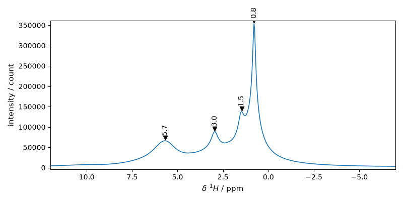
plot the position of the peaks For this we will define a plot function that we be reused later
def plot_with_pp(s, peaks):
    ax = s.plot()  # output the spectrum on ax. ax will receive next plot too;
    peak_offset = 0.02 * float(np.max(np.abs(np.asarray(s.data))))
    axis = np.asarray(s.x.data, dtype=float)
    point_pos = np.asarray(peaks.x.data, dtype=float).squeeze()
    peak_y = np.asarray(peaks.data, dtype=float).squeeze()
    peak_x = np.interp(point_pos, np.arange(s.shape[-1], dtype=float), axis)
    marker_y = peak_y + peak_offset

    ax.scatter(
        peak_x,
        marker_y,
        marker="v",
        color="black",
    )
    for x, y in zip(peak_x, marker_y, strict=False):
        ax.annotate(
            f"{x:0.1f}",
            xy=(x, y),
            xytext=(-5, 5),
            rotation=90,
            textcoords="offset points",
        )


def peak_positions_and_heights(s, peaks):
    axis = np.asarray(s.x.data, dtype=float)
    point_pos = np.asarray(peaks.x.data, dtype=float).squeeze()
    peak_y = np.asarray(peaks.data, dtype=float).squeeze()
    peak_x = np.interp(point_pos, np.arange(s.shape[-1], dtype=float), axis)
    order = np.argsort(peak_x)
    return peak_x[order], peak_y[order]


def build_fit_script(s, peaks):
    peak_x, peak_y = peak_positions_and_heights(s, peaks)
    lines = [
        "#-----------------------------------------------------------",
        "# Automatically initialized from the currently selected peaks",
        "#-----------------------------------------------------------",
        "",
        "COMMON:",
        "$ commonwidth: 0.2, 0.01, 1.0",
        "$ commonratio: .5, 0, 1",
        "",
    ]
    for i, (x, y) in enumerate(zip(peak_x, peak_y, strict=False), start=1):
        lines.extend(
            [
                f"MODEL: LINE_{i}",
                "shape: voigtmodel",
                f"    $ ampl:  {y:0.1f}, 0.0, none",
                f"    $ pos:   {x:0.4f}, {x - 0.25:0.4f}, {x + 0.25:0.4f}",
                "    > ratio: commonratio",
                "    > width: commonwidth",
                "",
            ]
        )
    return "\n".join(lines)


plot_with_pp(spectrum, peaks)
Set some parameters to get less but significant peaks
Peak fitting
Fit parameters are initialized from the currently selected peaks.
We will work here on the processed 1D region of interest.
create an Optimize object
f1 = scp.Optimize(log_level="INFO")
Set parameters
f1.script = script
f1.max_iter = 30000
Fit the slice s4p
**************************************************
Result:
**************************************************

COMMON:
       $ commonwidth:     0.7158, 0.01, 1.0
       $ commonratio:     0.0044, 0.0, 1.0

MODEL: line_1
shape: voigtmodel
       $ ampl: 249461.1389, 0.0, none
       $ pos:     0.8015, 0.5382, 1.0382
       > ratio:commonratio
       > width:commonwidth

MODEL: line_2
shape: voigtmodel
       $ ampl: 54074.9838, 0.0, none
       $ pos:     1.6306, 1.2289, 1.7289
       > ratio:commonratio
       > width:commonwidth

MODEL: line_3
shape: voigtmodel
       $ ampl: 61594.9205, 0.0, none
       $ pos:     2.9737, 2.7041, 3.2041
       > ratio:commonratio
       > width:commonwidth

MODEL: line_4
shape: voigtmodel
       $ ampl: 65076.0085, 0.0, none
       $ pos:     5.7166, 5.4338, 5.9338
       > ratio:commonratio
       > width:commonwidth
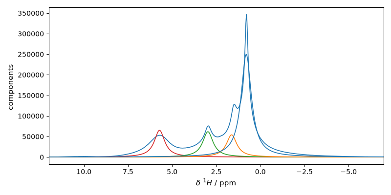
Show the result
_ = s4p.plot()
ax = (f1.components[:]).plot(clear=False)
ax.autoscale(enable=True, axis="y")

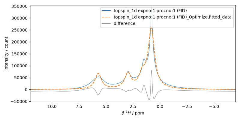
# Plotmerit
som = f1.inverse_transform()
_ = f1.plot_merit(offset=2)
This ends the example ! The following line can be removed or commented
when the example is run as a notebook (ipynb).
# scp.show()
Total running time of the script: ( 0 minutes 2.004 seconds)