NDDataset PCA analysis example

In this example, we perform the PCA dimensionality reduction of a spectra dataset

Import the spectrochempy API package

import spectrochempy as scp

Load a dataset

dataset = scp.read_omnic("irdata/nh4y-activation.spg")
dataset = dataset[:, 2000.0:4000.0]  # remember float number to slice from coordinates
print(dataset)
dataset.plot_stack()

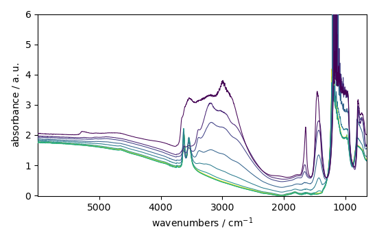
NDDataset: [float64] a.u. (shape: (y:55, x:2075))

<_Axes: xlabel='wavenumbers $\\mathrm{/\\ \\mathrm{cm}^{-1}}$', ylabel='absorbance $\\mathrm{/\\ \\mathrm{a.u.}}$'>

Create a PCA object

pca = scp.PCA(dataset, centered=False)

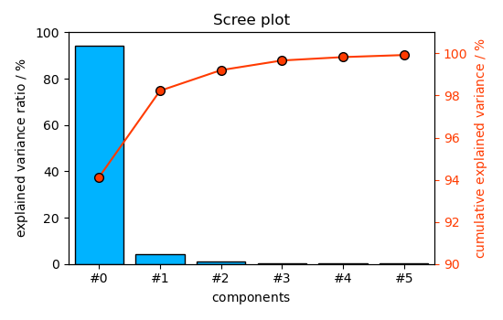
Reduce the dataset to a lower dimensionality (number of components is automatically determined)

S, LT = pca.reduce(n_pc=0.99)

print(LT)

NDDataset: [float64] a.u. (shape: (y:2, x:2075))

Finally, display the results graphically ScreePlot

_ = pca.screeplot()

• 
• 

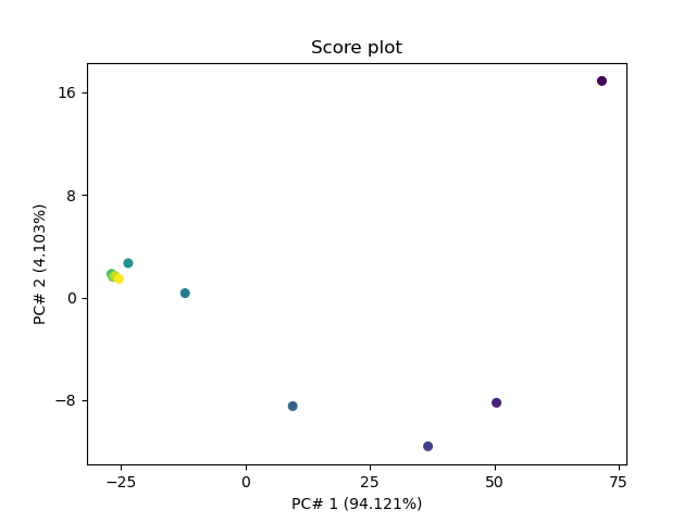
Score Plot

_ = pca.scoreplot(1, 2)

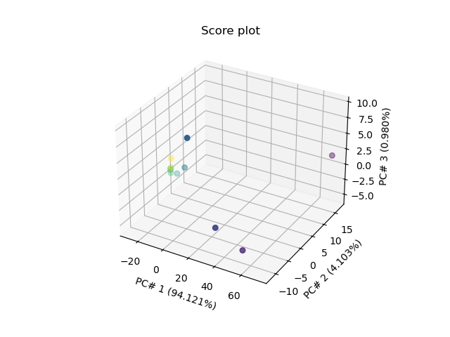
Score Plot for 3 PC’s in 3D

_ = pca.scoreplot(1, 2, 3)

Our dataset has already two columns of labels for the spectra but there are little too long for display on plots.

S.y.labels

array([[  2016-07-06 19:03:14+00:00,   vz0466.spa, Wed Jul 06 21:00:38 2016 (GMT+02:00)],
       [  2016-07-06 19:13:14+00:00,   vz0467.spa, Wed Jul 06 21:10:38 2016 (GMT+02:00)],
       ...,
       [  2016-07-07 04:03:17+00:00,   vz0520.spa, Thu Jul 07 06:00:41 2016 (GMT+02:00)],
       [  2016-07-07 04:13:17+00:00,   vz0521.spa, Thu Jul 07 06:10:41 2016 (GMT+02:00)]], dtype=object)

So we define some short labels for each component, and add them as a third column:

labels = [lab[:6] for lab in dataset.y.labels[:, 1]]
# we cannot change directly the label as S is read-only, but use the method `labels`
pca.labels(labels)  # Note this does not replace previous labels, but adds a column.

now display thse

_ = pca.scoreplot(1, 2, show_labels=True, labels_column=2, labels_every=5)

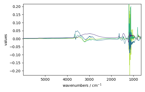
Displays the 4-first loadings

LT[:4].plot_stack()

scp.show()  # uncomment to show plot if needed (not necessary in jupyter notebook)