Note
Go to the end to download the full example code
2D-IRIS analysis example
In this example, we perform the 2D IRIS analysis of CO adsorption on a sulfide catalyst.
import spectrochempy as scp
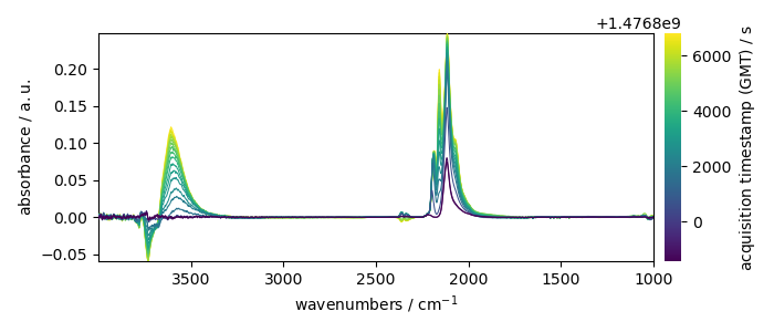
Uploading dataset
X has two coordinates:
* wavenumbers named “x”
* and timestamps (i.e., the time of recording) named “y”.
print(X.coordset)
CoordSet: [x:wavenumbers, y:acquisition timestamp (GMT)]
Setting new coordinates
The y coordinates of the dataset is the acquisition timestamp.
However, each spectrum has been recorded with a given pressure of CO
in the infrared cell.
Hence, it would be interesting to add pressure coordinates to the y dimension:
pressures = [
    0.003,
    0.004,
    0.009,
    0.014,
    0.021,
    0.026,
    0.036,
    0.051,
    0.093,
    0.150,
    0.203,
    0.300,
    0.404,
    0.503,
    0.602,
    0.702,
    0.801,
    0.905,
    1.004,
]

c_pressures = scp.Coord(pressures, title="pressure", units="torr")
Now we can set multiple coordinates:
CoordSet: [_1:acquisition timestamp (GMT), _2:pressure]
To get a detailed a rich display of these coordinates. In a jupyter notebook, just type:
By default, the current coordinate is the first one (here c_times).
For example, it will be used by default for
plotting:
prefs = X.preferences
prefs.figure.figsize = (7, 3)
_ = X.plot(colorbar=True)
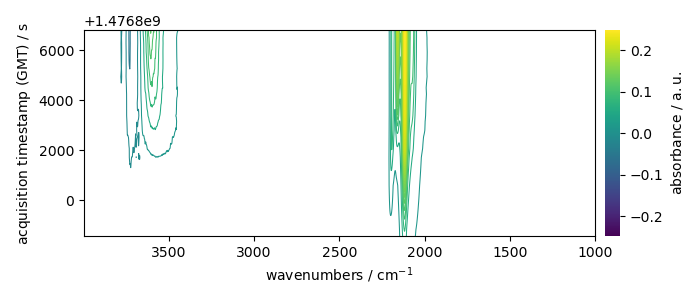
_ = X.plot_map(colorbar=True)
To seamlessly work with the second coordinates (pressures), we can change the default coordinate:
X.y.select(2)  # to select coordinate ``_2``
X.y.default
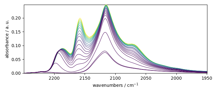
Let’s now plot the spectral range of interest. The default coordinate is now used:
X_ = X[:, 2250.0:1950.0]
print(X_.y.default)
_ = X_.plot()
_ = X_.plot_map()
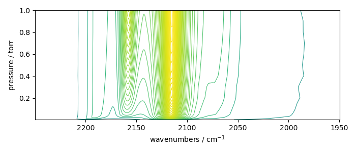
Coord: [float64] torr (size: 19)
IRIS analysis without regularization
%%
Perform IRIS without regularization (the loglevel can be set to INFO to have
information on the running process)
scp.set_loglevel(scp.INFO)
iris = scp.IRIS(X_, "langmuir", q=[-8, -1, 50])
Build kernel matrix with: langmuir

Build S matrix (sharpness)

... done

Solving for 312 channels and 19 observations, no regularization

-->  residuals = 1.09e-01    curvature = 9.15e+04

Done.
Plots the results
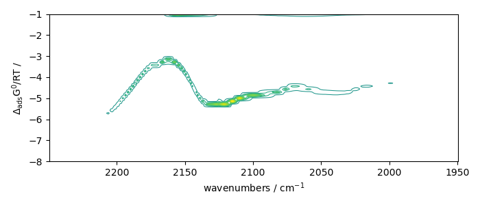

With regularization and a manual search
%% Perform IRIS with regularization, manual search
iris = scp.IRIS(X_, "langmuir", q=[-8, -1, 50], reg_par=[-10, 1, 12])
iris.plotlcurve(title="L curve, manual search")
iris.plotdistribution(-7)
_ = iris.plotmerit(-7)
Build kernel matrix with: langmuir

Build S matrix (sharpness)

... done

Solving for 312 channels, 19 observations and 12 regularization parameters

log10(lambda)=-10.000 -->  residuals = 1.088e-01    regularization constraint  = 9.085e+04

log10(lambda)=-9.000 -->  residuals = 1.088e-01    regularization constraint  = 8.266e+04

log10(lambda)=-8.000 -->  residuals = 1.093e-01    regularization constraint  = 2.244e+04

log10(lambda)=-7.000 -->  residuals = 1.104e-01    regularization constraint  = 3.301e+03

log10(lambda)=-6.000 -->  residuals = 1.121e-01    regularization constraint  = 6.108e+02

log10(lambda)=-5.000 -->  residuals = 1.153e-01    regularization constraint  = 1.148e+02

log10(lambda)=-4.000 -->  residuals = 1.210e-01    regularization constraint  = 2.192e+01

log10(lambda)=-3.000 -->  residuals = 1.309e-01    regularization constraint  = 4.383e+00

log10(lambda)=-2.000 -->  residuals = 1.474e-01    regularization constraint  = 9.509e-01

log10(lambda)=-1.000 -->  residuals = 1.778e-01    regularization constraint  = 3.208e-01

log10(lambda)=0.000 -->  residuals = 2.639e-01    regularization constraint  = 1.399e-01

log10(lambda)=1.000 -->  residuals = 5.505e-01    regularization constraint  = 9.736e-02


Done.
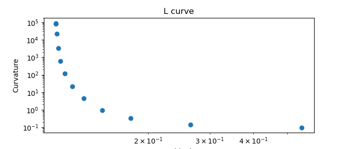
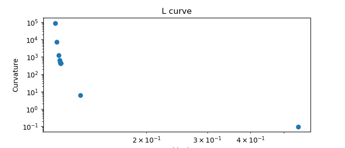
Automatic search
%% Now try an automatic search of the regularization parameter:
iris = scp.IRIS(X_, "langmuir", q=[-8, -1, 50], reg_par=[-10, 1])
iris.plotlcurve(title="L curve, automated search")
 Build kernel matrix with: langmuir

 Build S matrix (sharpness)

 ... done

 Solving for 312 channel(s) and 19 observations, search optimum regularization parameter in the range: [10**-10, 10**1]

 Initial Log(lambda) values = [     -10   -5.798   -3.202        1]
 log10(lambda)=-10.000 -->  residuals = 1.088e-01    regularization constraint  = 9.085e+04

 log10(lambda)=-5.798 -->  residuals = 1.126e-01    regularization constraint  = 4.325e+02

 log10(lambda)=-3.202 -->  residuals = 1.284e-01    regularization constraint  = 6.047e+00

 log10(lambda)=1.000 -->  residuals = 5.505e-01    regularization constraint  = 9.736e-02

 Curvatures of the inner points: C1 = 0.012 ; C2 = 0.163

 New range of Log(lambda) values: [     -10   -7.403   -5.798   -3.202]
 log10(lambda)=-7.403 -->  residuals = 1.099e-01    regularization constraint  = 7.236e+03

 new curvature: C2 = 0.014
 New range (Log lambda):[  -7.403   -5.798   -4.807   -3.202]
 log10(lambda)=-4.807 -->  residuals = 1.162e-01    regularization constraint  = 8.329e+01

 Curvatures of the inner points: C1 = 0.010 ; C2 = 0.021

 New range of Log(lambda) values: [  -7.403   -6.411   -5.798   -4.807]
 log10(lambda)=-6.411 -->  residuals = 1.113e-01    regularization constraint  = 1.223e+03

 new curvature: C2 = 0.012
 New range (Log lambda):[  -6.411   -5.798    -5.42   -4.807]
 log10(lambda)=-5.420 -->  residuals = 1.138e-01    regularization constraint  = 2.293e+02

 Curvatures of the inner points: C1 = 0.011 ; C2 = 0.014

 New range of Log(lambda) values: [  -6.411   -6.033   -5.798    -5.42]
 log10(lambda)=-6.033 -->  residuals = 1.121e-01    regularization constraint  = 6.458e+02

 new curvature: C2 = 0.012
 New range (Log lambda):[  -6.033   -5.798   -5.654    -5.42]
 log10(lambda)=-5.654 -->  residuals = 1.130e-01    regularization constraint  = 3.413e+02

 Curvatures of the inner points: C1 = 0.011 ; C2 = 0.013

 New range of Log(lambda) values: [  -6.033   -5.888   -5.798   -5.654]
 log10(lambda)=-5.888 -->  residuals = 1.124e-01    regularization constraint  = 5.035e+02

 new curvature: C2 = 0.013
 New range (Log lambda):[  -5.888   -5.798   -5.743   -5.654]
 log10(lambda)=-5.743 -->  residuals = 1.128e-01    regularization constraint  = 3.950e+02

 Curvatures of the inner points: C1 = 0.013 ; C2 = 0.015

 New range of Log(lambda) values: [  -5.888   -5.833   -5.798   -5.743]
 log10(lambda)=-5.833 -->  residuals = 1.126e-01    regularization constraint  = 4.582e+02

 new curvature: C2 = 0.013
 New range (Log lambda):[  -5.833   -5.798   -5.777   -5.743]
 log10(lambda)=-5.777 -->  residuals = 1.127e-01    regularization constraint  = 4.176e+02

 Curvatures of the inner points: C1 = 0.012 ; C2 = 0.015

 New range of Log(lambda) values: [  -5.833   -5.811   -5.798   -5.777]
 log10(lambda)=-5.811 -->  residuals = 1.126e-01    regularization constraint  = 4.421e+02

 new curvature: C2 = 0.011
 New range (Log lambda): [  -5.833   -5.819   -5.811   -5.798]
 log10(lambda)=-5.819 -->  residuals = 1.126e-01    regularization constraint  = 4.482e+02


 optimum found: index = 7 ; Log(lambda) = -5.811 ; lambda = 1.54375e-06 ; curvature = 0.012

 Done.

<Axes: title={'center': 'L curve'}, xlabel='Residuals', ylabel='Curvature'>
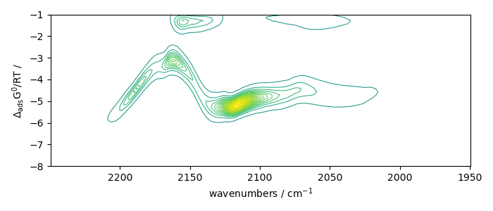
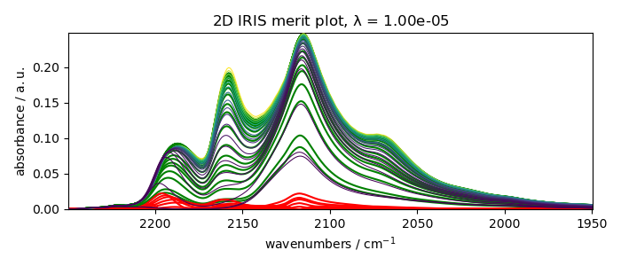
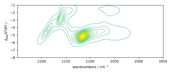
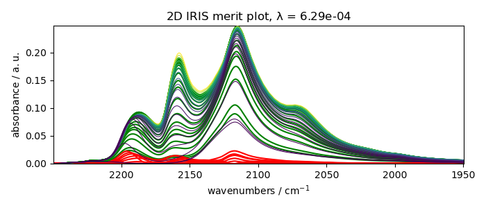
The data corresponding to the largest curvature of the L-curve are at the second last position of output data:
iris.plotdistribution(-2)
_ = iris.plotmerit(-2)

# scp.show()  # uncomment to show plot if needed (not necessary in jupyter notebook)
Total running time of the script: ( 0 minutes 24.730 seconds)