
Plot Types#
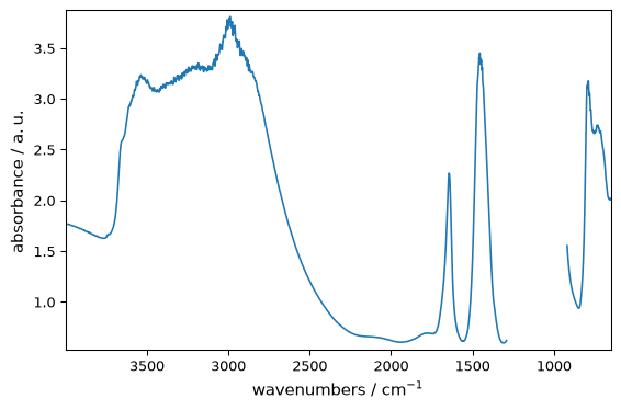
SpectroChemPy provides several plotting methods. ds.plot() chooses automatically, but explicit methods give you control.
ds.plot() uses the default geometry for the dataset dimensionality. Use the explicit helpers below when you want the intended rendering to be obvious from the code itself.
Line Plot#
For spectra and time-series:
[1]:
import os
from pathlib import Path

import spectrochempy as scp

TEST_FILE = Path(os.environ.get("TEST_FILE", "irdata/nh4y-activation.spg"))

ds = scp.read(TEST_FILE)
ds = ds[:, 4000.0:650.0]  # We keep only the region that we want to display
ds.y -= ds.y[0]  # Set y coordinates as relative time  for better visualization
ds.y.ito("hour")
ds.y.title = "Time on stream"  # Update y-axis title accordingly
ds[:, 1290.0:920.0] = scp.MASKED  # We also mask a region that we do not want to display
ds1 = ds[0]  # Single spectrum
[2]:
_ = ds1.plot()
The explicit 1D helpers are:
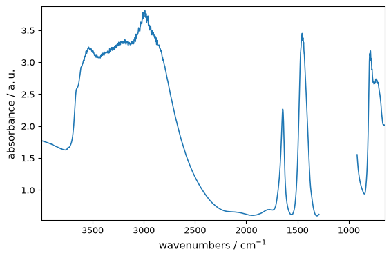
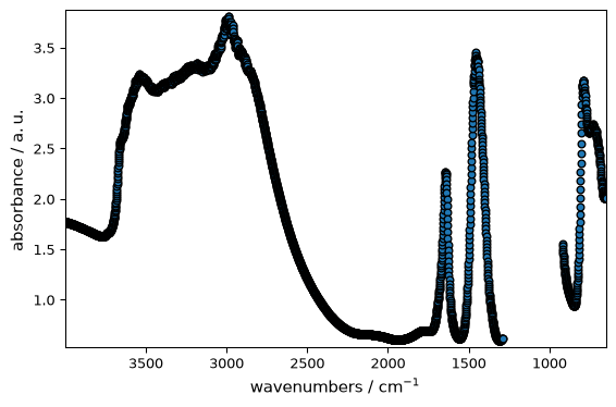
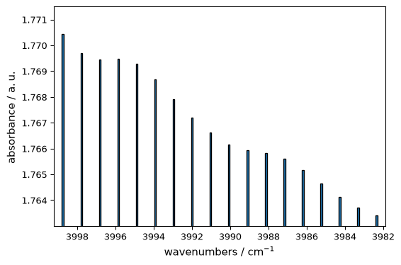
plot_pen()for line plots,plot_scatter()for marker-based plots,plot_bar()for bar charts.
scatter=True is still accepted for compatibility, but plot_scatter() or method="scatter" is clearer in new code.
[3]:
_ = ds1.plot_pen()
[4]:
_ = ds1.plot_scatter(ms=5)
[5]:
_ = ds1[:20].plot_bar()
Or using plot_lines() explicitly (canonical form):
[6]:
_ = ds.plot_lines()
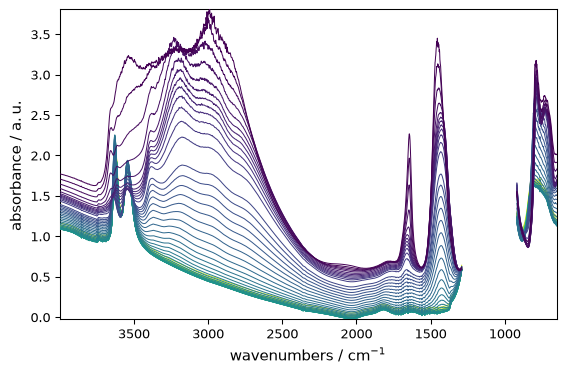
Image Plot#
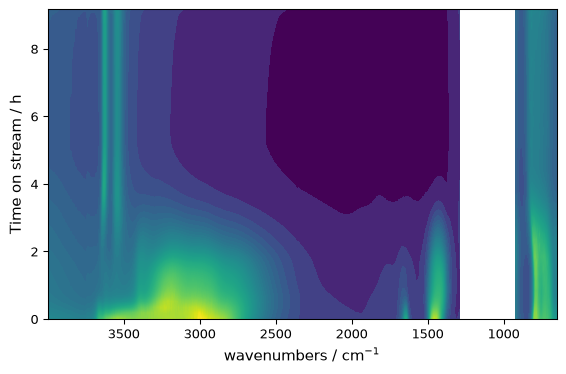
For 2D data where both axes are numerical:
[7]:
_ = ds.plot_image()
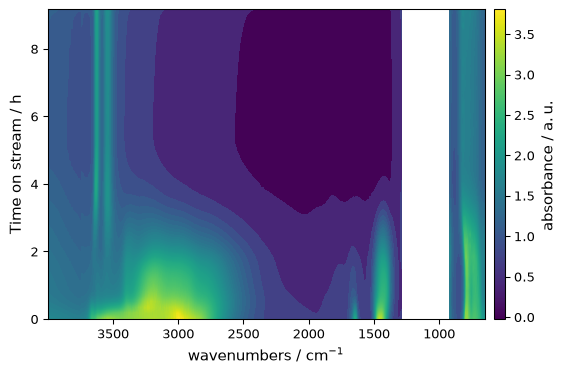
Request a colorbar when you want the intensity scale to be explicit:
[8]:
_ = ds.plot_image(colorbar=True)
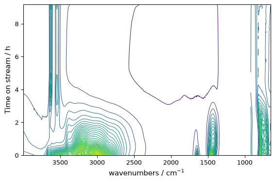
Contour Plot#
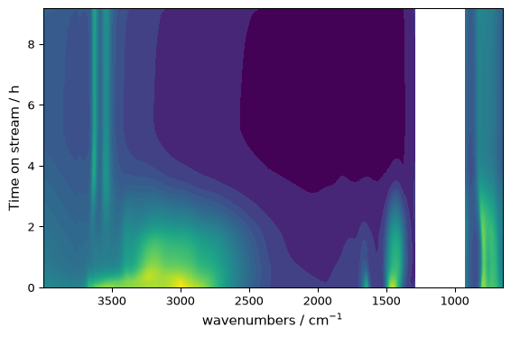
For continuous data with smooth transitions:
[9]:
_ = ds.plot_contour()
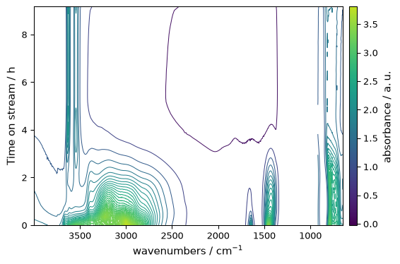
Contour plots also support colorbars:
[10]:
_ = ds.plot_contour(colorbar=True)
Calculated Projections#
Add marginal curves by naming the dimensions to retain. In this time-series dataset, x is wavenumber and y is time. The top panel retains x and reduces over time; the right panel retains y and reduces over wavenumber.
The reducers sum, mean and max exclude masked and non-finite samples. These are pointwise reductions, not coordinate-weighted integrals: on an irregular grid, a sum is not the area under a spectrum.
[11]:
_ = ds.plot_contour(
    projections=("x", "y"),
    projection_reducer="mean",
    projection_size=0.25,
    colorbar=True,
    figsize=(8, 5),
)
projections=True selects both dimensions and False disables them for that call. If omitted, the show_projections and show_projection_x/y preferences apply. Names keep their numerical meaning after transposition: ds.T.plot_contour(projections="x") puts the retained wavenumber dimension on the right because it is now the vertical axis.
To show measured spectra instead of reductions of the map, supply projection_data. The advanced plotting tutorial shows external references, signed contours and complete multi-panel figures.
Filled Contour / Image-like Plot#
For image-like filled rendering, use plot_contourf() or plot_image():
[12]:
_ = ds.plot_contourf(colorbar=True)

Decision Guide#
Method |
Use When |
|---|---|
|
Showing spectra, time series, or stacked traces |
|
Explicit 1D line, marker, or bar rendering |
|
2D field with spatial x/y axes |
|
Smooth visualization of continuous 2D data |
|
Filled, image-like contour rendering |
|
3D perspective view of 2D data |
|
3D-style waterfall representation |
Surface Plot#
For a 3D perspective view of 2D data:
[13]:
_ = ds.plot_surface(y_reverse=True, linewidth=0)

Waterfall Plot#
For a waterfall-style representation:
[14]:
_ = ds.plot_waterfall(y_reverse=True, figsize=(6, 5))

Overlay Several Datasets on One Axes#
plot_multiple() overlays several 1D datasets on the same Matplotlib axes. Use it when you want one shared set of axes and one combined legend.
[15]:
datasets = [ds[0], ds[5], ds[10]]
_ = scp.plot_multiple(
    datasets,
    method="scatter",
    labels=["t0", "t5", "t10"],
    legend="best",
    ms=4,
)

Arrange Several Datasets on a Grid#
multiplot() creates a grid of axes. Use it when each dataset should keep its own panel rather than being overlaid.
[16]:
_ = scp.multiplot([ds[0], ds[5], ds[10], ds[15]], nrows=2, ncols=2, method="pen")

Combining with Options#
All plot methods accept the same customization options:
[17]:
_ = ds.plot_image(
    cmap="plasma",
    xlim=(2000, 1300),
    ylim=(1, 5),
)

The appropriate method is chosen automatically when you call ds.plot(), but explicit methods make your intent clear and provide specific functionality.
Deprecated Method Names#
The following legacy names still work, but the canonical names are preferred for new code:
Legacy name |
Preferred name |
|---|---|
|
|
|
|
plot_image() is not deprecated: it remains a supported explicit helper for image-style plotting, alongside plot_contourf(). Choose the name that makes your intent clearer.