Warning

You are reading the documentation related to the development version. Go here if you are looking for the documentation of the stable release.

Filtering, Smoothing and Denoising

In this tutorial, we show how to filter/smooth 1D and 2D spectra and gives information on the algorithms used in Spectrochempy.

We first import spectrochempy, the other libraries used in this tutorial, and a sample raman dataset:

import spectrochempy as scp

SpectroChemPy's API - v.0.6.9.dev9 © Copyright 2014-2024 - A.Travert & C.Fernandez @ LCS

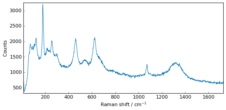
First, we import a sample raman spectrum:

# use the generic read function. Note that read_labspec would be equivalent for this file format.
X = scp.read("ramandata/labspec/SMC1-Initial_RT.txt")

and plot it:

# Use preferences to set the figure size for all figures
prefs = X.preferences
prefs.figure.figsize = (8, 4)

# and use plot method of the NDDataset
_ = X.plot()

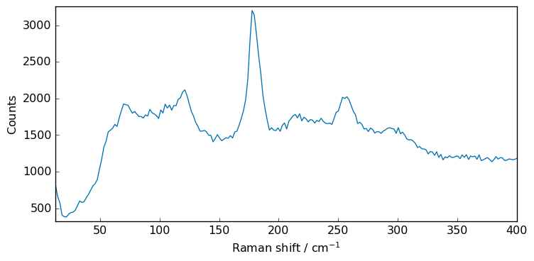
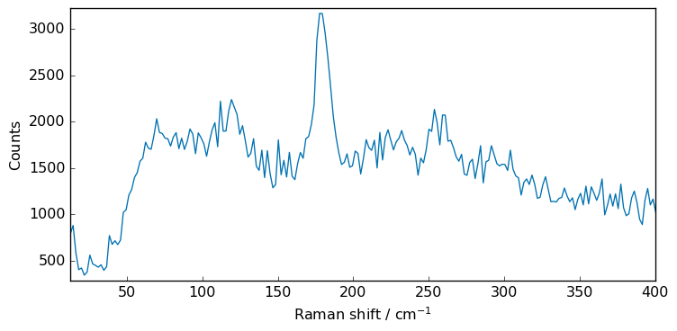
To have a better view of the filters effect, we will zoom on a smaller region: (0,400) cm\(^{-1}\) and we will add some additional noise.

# select a region by slicing (note the original shape is (1, 1024)
Xs = X[:, 0.0:400.0]
print("shape: ", X.shape)
_ = Xs.plot()

shape:  (1, 1024)

import numpy as np

noise = np.random.normal(0, 100, 215)
Xn = Xs + noise
_ = Xn.plot()

The Filter processor

The Filter processor is a generic processor which can be used to filter 1D and 2D spectra.

Here is a demonstration on how to use it to smooth a 1D spectrum.

Moving average

In its simplest form of smoothing is a unweighted moving average - each absorbance at a given wavenumber of the smoothed spectrum is the average of the absorbance at the absorbance at the considered wavenumber and the N neighboring wavenumbers (i.e. N/2 before and N/2 after), hence the conventional use of an odd number of N+1 points to define the window length. For the points located at both end of the spectra, the extremities of the spectrum are mirrored beyond the initial limits to minimize boundary effects.

Let’s create a filter processor with a moving average (method avg) of 3 points (default size is 5).

filter = scp.Filter(method="avg", size=5)

Apply the filter to the spectrum Xn

Xsm = filter.transform(Xn)

Note that the above syntax can be simplified to the equivalent:

Xsm = filter(Xn)

Now, let’s plot the result.

However, as this will be repeated along the tutorial, we first make a function to plot both original and transformed spectra on the same figure, with a legend.

def plot(X, Xm, label=None, xlim=None):
    X.plot(color="b", label="original")
    ax = Xm.plot(clear=False, color="r", ls="-", lw=1.5, label=label)
    diff = X - Xm
    s = round(diff.std(dim=-1).values, 2)
    ax = diff.plot(clear=False, ls="-", lw=1, label=f"difference (std={s})")
    ax.legend(loc="best", fontsize=10)
    if xlim is not None:
        ax.set_xlim(xlim)
    scp.show()

plot(Xn, Xsm, label="Moving average (5 points)")

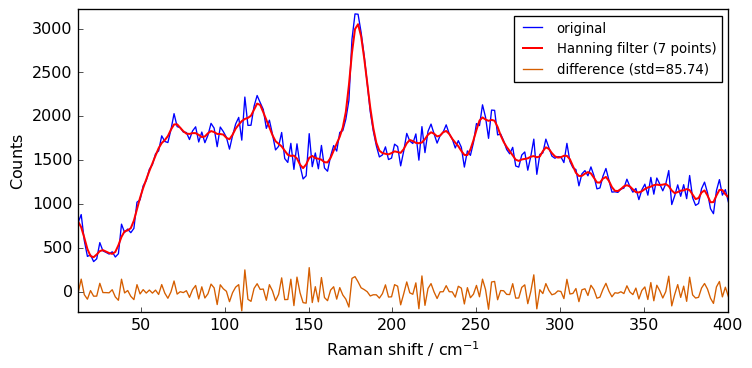
Convolution with window filters

These filters are based on the convolution of scaled window, with the signal. For instance the han convolution method use a han (also known as ‘hanning’) window.

filter = scp.Filter(
    method="han", size=7
)  # can also be one of 'hamming', 'bartlett', # 'blackman'.
Xhan = filter(Xn)
plot(Xn, Xhan, label="Hanning filter (7 points)")

Savitzky-Golay filter

The Filter processor can also be used to apply a Savitzky-Golay filter to the spectrum.

This algorithm uses a polynomial interpolation in the moving window. A demonstrative illustration of the method can be found on the Savitzky-Golay filter entry of Wikipedia.

The function implemented in spectrochempy is a wrapper of the savgol_filter() method from the scipy.signal module to which we refer the interested reader. It not only used to smooth spectra but also to compute their successive derivatives. The latter are treated in the peak-finding tutorial and we will focus here on the smoothing which is the default of the filter (default parameter: deriv=0 ).

As for the previous kernel-based filters, it is a moving-window based method. Hence, the window length (size parameter) plays an equivalent role. Moreover, instead of choosing a window function, the user can choose the order of the polynomial used to fit the window data points (order , default value: 0). The latter must be strictly smaller than the window size (so that the polynomial coefficients can be fully determined).

filter = scp.Filter(
    method="savgol", size=5, order=0
)  # default is size=5, order=2, deriv=0
Xsgs = filter(Xn)
plot(Xn, Xsgs, label="Savitzky-Golay (5 points, order=0)")

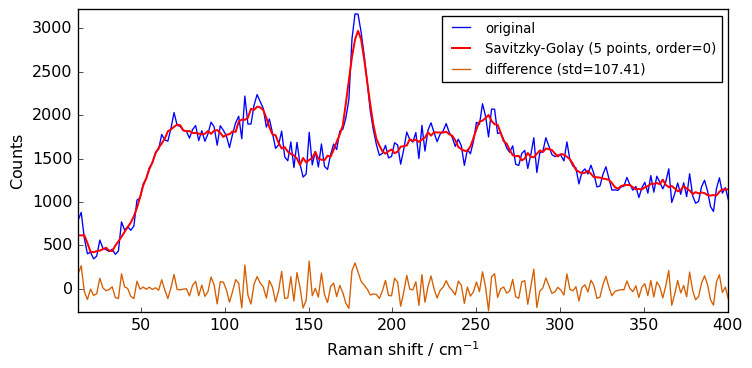
As the order is set to 0, there is no much difference compared to a simple moving average.

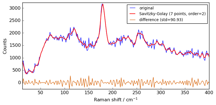
Now we can try to increase the polynomial order to 2 to see the effect on the smoothing.

filter.order = 2
filter.size = 7
Xsm2 = filter(Xn)
plot(Xn, Xsm2, label="Savitzky-Golay (7 points, order=2)")

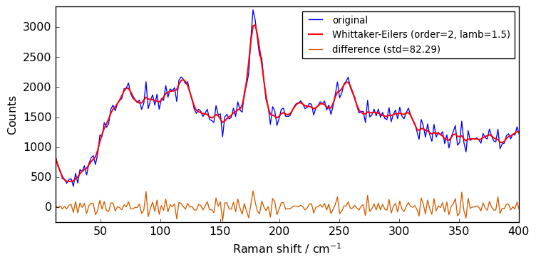
Whittaker-Eilers filter

As good alternative to the Savitzky-Golay filter want can choose to use the Whittaker-Eilers smoother described in: P. H. C. Eilers, “A perfect smoother”, Anal. Chem. 2003, 75, 3631-3636. The implementation in SpectroChemPy is based on the work by H. V. Werts (https://github.com/mhvwerts/whittaker-eilers-smoother). The main parameter to be changed is the lamb (‘λ’ in the Eilers paper), which determines the strength of the smoothing. Note that it may needs tuning over several orders of magnitude (1, 10, 100, 1000, …).

filter = scp.Filter(method="whittaker", order=2, lamb=1.5)
Xwhit = filter(Xn)
plot(Xn, Xwhit, label="Whittaker-Eilers (order=2, lamb=1.5)")

Filtering using API or NDDataset methods.

In addition to the Filter processor which provide an uniform interface to the various filter methods provided by SpectroChemPy, it is also possible (as in previous version of spectrochempy) to use specific NDDataset methods or API functions.

Let’s demonstrate this here.

The smooth method

When simply used as this, i.e. X.smooth() , the method uses a default moving average (‘avg’) of 5 points:

Xsm = Xn.smooth()  # NDDataset method

Note that it is also possible to use the API function scp.smooth(X) instead of the dataset method X.smooth(). The result is the same.

Xsm = scp.smooth(Xn)  # SpectroChemPy API function

Window size influence

The following code compares the influence of the window size on the smoothing of the Xn NDDataset.

for size in [3, 5, 7, 9, 11]:
    Xsm = Xn.smooth(size)
    plot(Xn, Xsm, label=f"smooth `avg` size={size}")

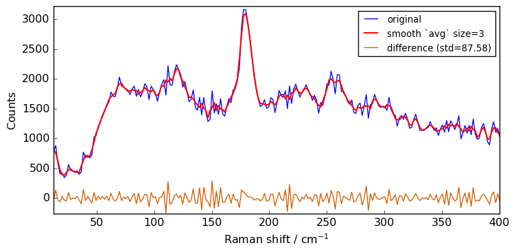
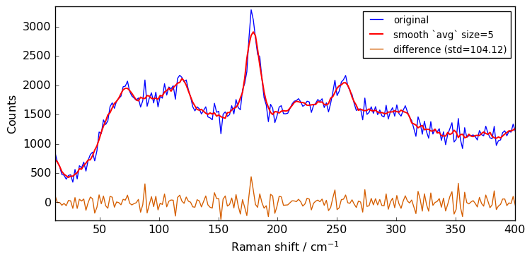
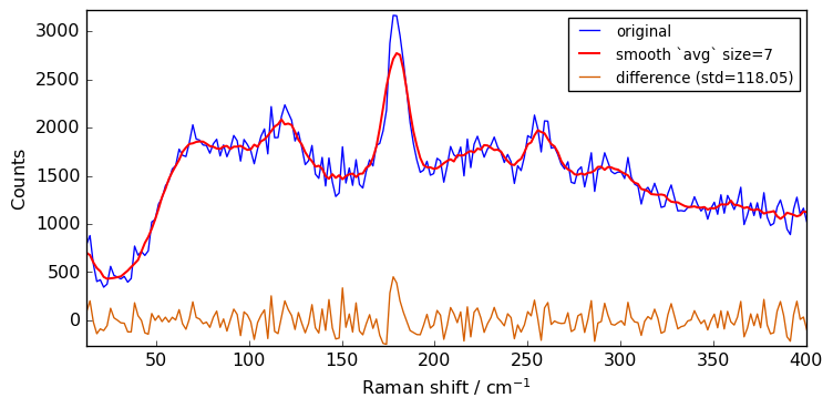
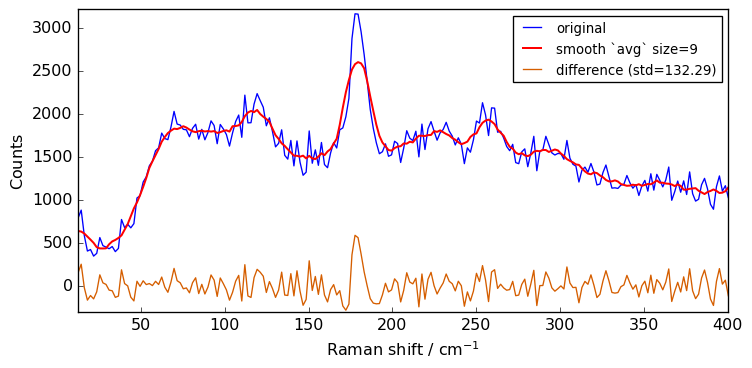
The above spectra clearly show that for large value of the size parameter, the spectrum is flattened out and distorted.

When determining the optimum window size, one should thus consider the balance between noise removal and signal integrity: the larger the window size, the stronger the smoothing, but also the greater the chance to distort the spectrum.

Convolution with windows

Besides the window size, the user can also choose the type of window (window ) from flat(eq. to avg) , han , hamming , bartlett or blackman . The flat window - which is the default shown above - should be fine for the vast majority of cases.

The code below compares the effect of the type of window:

size = 7
for window in ["flat", "bartlett", "han", "hamming", "blackman"]:
    Xsm = Xn.smooth(size=size, window=window)
    plot(Xn, Xsm, label=f"window=`{window}` size={size}")

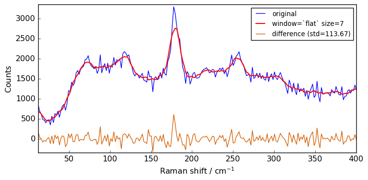
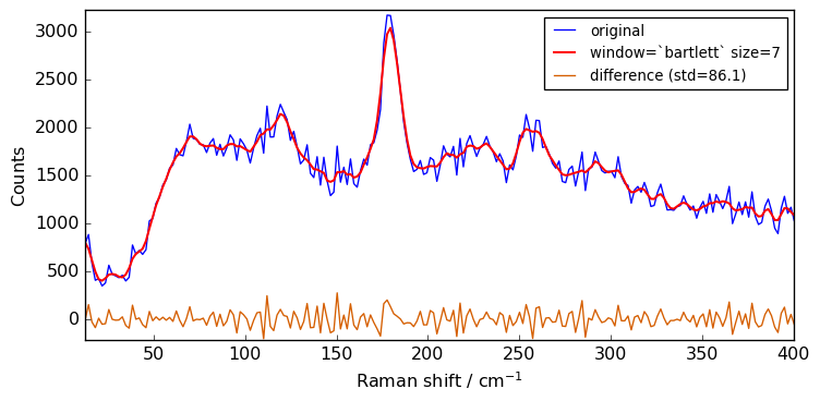
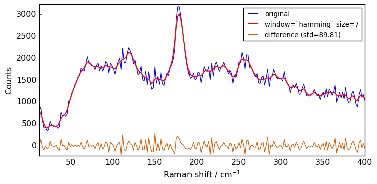
Close examination of the spectra shows that the flat window leads to the stronger smoothing. This is because the other window functions are used as weighting functions for the N+1 points, with the largest weight on the central point and smaller weights for external points.

The window functions as used in SpectroChemPy are derived from the scipy library. These builtin functions are such that the value of the central point is 1. Hence, as shown below, they are normalized to the sum of weights. The code below displays the corresponding normalized functions for size=27 points:

import numpy as np
import scipy

functions = []
labels = []
size = 27
for i, method in enumerate(["bartlett", "han", "hamming", "blackman"]):
    data = scipy.signal.get_window(method, size, fftbins=False)
    data = data / np.sum(data)

    s = scp.NDDataset(
        data + 0.02 * i
    )  # normalized window function, y shifted : +0.1 for each function
    functions.append(s)
    labels.append(f"function: {method}")

ax = scp.plot_multiple(
    figsize=(8, 5),  # ylim=(0,0.1),
    method="pen",
    datasets=functions,
    labels=labels,
    ls="-",
    lw=2,
)
_ = ax.legend(labels, loc="upper left", fontsize=10)

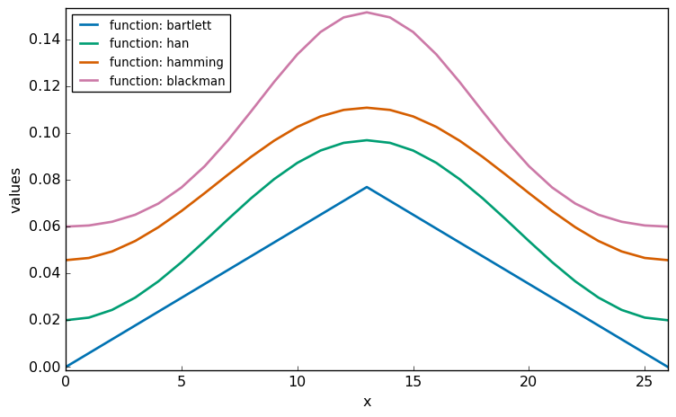
As shown above, the “bartlett” function is equivalent to a triangular window, while other functions (hanning , hamming , blackman ) are bell-shaped. More information on window functions can be found here.

Savitzky-Golay filter:savgol

Similarly, the Savitsky-Golay filter is also implemented as an API/NDDataset method:

Xsg = scp.savgol(Xn, size=5, order=2, mode="mirror")

Whittaker-eilers filter : whittaker

Finally, we can also use the whittaker filter directly. e.g.:

Xw = scp.whittaker(Xn, lamb=10)