Warning

You are reading the documentation related to the development version. Go here if you are looking for the documentation of the stable release.

Mathematical operations

import numpy as np

import spectrochempy as scp
from spectrochempy import MASKED, DimensionalityError, error_

SpectroChemPy's API - v.0.6.9.dev9 © Copyright 2014-2024 - A.Travert & C.Fernandez @ LCS

Ufuncs (Universal Numpy’s functions)

A universal function (or ufunc in short) is a function that operates on numpy arrays in an element-by-element fashion, supporting array broadcasting, type casting, and several other standard features. That is, a ufunc is a “vectorized” wrapper for a function that takes a fixed number of specific inputs and produces a fixed number of specific outputs.

For instance, in numpy to calculate the square root of each element of a given nd-array, we can write something like this using the np.sqrt functions :

x = np.array([1.0, 2.0, 3.0, 4.0, 6.0])
np.sqrt(x)

array([       1,    1.414,    1.732,        2,    2.449])

As seen above, np.sqrt(x) return a numpy array.

The interesting thing, it that ufunc’s can also work with NDDataset .

dx = scp.NDDataset(x)
np.sqrt(dx)

name	NDDataset_4dcb3d58
author	runner@fv-az1501-19
created	2024-04-28 03:11:55+02:00
history	2024-04-28 03:11:55+02:00> Ufunc sqrt applied.
DATA
title	sqrt()
values	[ 1 1.414 1.732 2 2.449]
size	5

List of UFuncs working on NDDataset:

Functions affecting magnitudes of the number but keeping units

• negative(x, **kwargs): Numerical negative, element-wise.

• absolute(x, **kwargs): Calculate the absolute value, element-wise. Alias: abs

• fabs(x, **kwargs): Calculate the absolute value, element-wise. Complex values are not handled, use absolute to find the absolute values of complex data.

• conj(x, **kwargs): Return the complex conjugate, element-wise.

• rint(x, **kwargs) :Round to the nearest integer, element-wise.

• floor(x, **kwargs): Return the floor of the input, element-wise.

• ceil(x, **kwargs): Return the ceiling of the input, element-wise.

• trunc(x, **kwargs): Return the truncated value of the input, element-wise.

Functions affecting magnitudes of the number but also units

• sqrt(x, **kwargs): Return the non-negative square-root of an array, element-wise.

• square(x, **kwargs): Return the element-wise square of the input.

• cbrt(x, **kwargs): Return the cube-root of an array, element-wise.

• reciprocal(x, **kwargs): Return the reciprocal of the argument, element-wise.

Functions that require no units or dimensionless units for inputs. Returns dimensionless objects.

• exp(x, **kwargs): Calculate the exponential of all elements in the input array.

• exp2(x, **kwargs): Calculate 2**p for all p in the input array.

• expm1(x, **kwargs): Calculate exp(x) - 1 for all elements in the array.

• log(x, **kwargs): Natural logarithm, element-wise.

• log2(x, **kwargs): Base-2 logarithm of x.

• log10(x, **kwargs): Return the base 10 logarithm of the input array, element-wise.

• log1p(x, **kwargs): Return log(x + 1) , element-wise.

Functions that return numpy arrays (Work only for NDDataset)

• sign(x): Returns an element-wise indication of the sign of a number.

• logical_not(x): Compute the truth value of NOT x element-wise.

• isfinite(x): Test element-wise for finiteness.

• isinf(x): Test element-wise for positive or negative infinity.

• isnan(x): Test element-wise for NaN and return result as a boolean array.

• signbit(x): Returns element-wise True where signbit is set.

Trigonometric functions. Require unitless data or radian units.

• sin(x, **kwargs): Trigonometric sine, element-wise.

• cos(x, **kwargs): Trigonometric cosine element-wise.

• tan(x, **kwargs): Compute tangent element-wise.

• arcsin(x, **kwargs): Inverse sine, element-wise.

• arccos(x, **kwargs): Trigonometric inverse cosine, element-wise.

• arctan(x, **kwargs): Trigonometric inverse tangent, element-wise.

Hyperbolic functions

• sinh(x, **kwargs): Hyperbolic sine, element-wise.

• cosh(x, **kwargs): Hyperbolic cosine, element-wise.

• tanh(x, **kwargs): Compute hyperbolic tangent element-wise.

• arcsinh(x, **kwargs): Inverse hyperbolic sine element-wise.

• arccosh(x, **kwargs): Inverse hyperbolic cosine, element-wise.

• arctanh(x, **kwargs): Inverse hyperbolic tangent element-wise.

Unit conversions

• deg2rad(x, **kwargs): Convert angles from degrees to radians.

• rad2deg(x, **kwargs): Convert angles from radians to degrees.

Binary Ufuncs

• add(x1, x2, **kwargs): Add arguments element-wise.

• subtract(x1, x2, **kwargs): Subtract arguments, element-wise.

• multiply(x1, x2, **kwargs): Multiply arguments element-wise.

• divide or true_divide(x1, x2, **kwargs): Returns a true division of the inputs, element-wise.

• floor_divide(x1, x2, **kwargs): Return the largest integer smaller or equal to the division of the inputs.

• mod or remainder(x1, x2,**kwargs): Return element-wise remainder of division.

• fmod(x1, x2, **kwargs): Return the element-wise remainder of division.

Usage

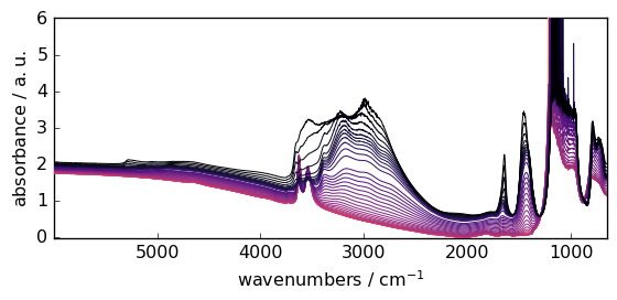
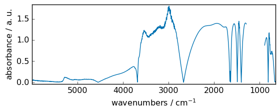
To demonstrate the use of mathematical operations on spectrochempy object, we will first load an experimental 2D dataset.

d2D = scp.read_omnic("irdata/nh4y-activation.spg")
prefs = d2D.preferences
prefs.colormap = "magma"
prefs.colorbar = False
prefs.figure.figsize = (6, 3)
_ = d2D.plot()

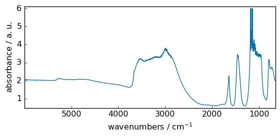
Let’s select only the first row of the 2D dataset ( the squeeze method is used to remove the residual size 1 dimension). In addition, we mask the saturated region.

dataset = d2D[0].squeeze()
_ = dataset.plot()

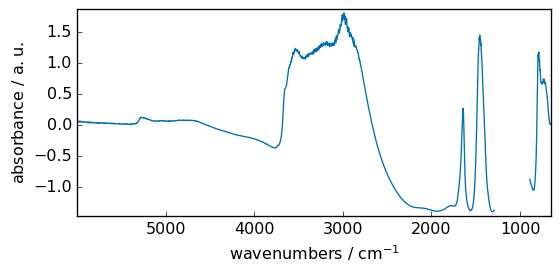
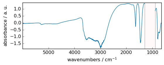
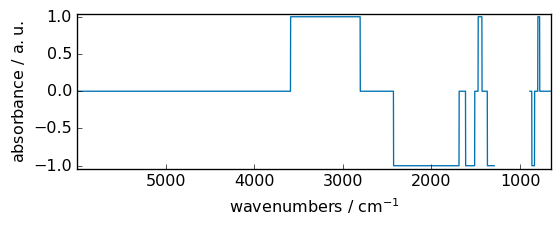
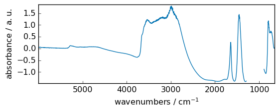
This dataset will be artificially modified already using some mathematical operation (subtraction with a scalar) to present negative values, and we will also mask some data

dataset -= 2.0  # add an offset to make that some of the values become negative
dataset[1290.0:890.0] = scp.MASKED  # additionally we mask some data
_ = dataset.plot()

Unary functions

Functions affecting magnitudes of the number but keeping units

negative

Numerical negative, element-wise, keep units

out = np.negative(dataset)  # the same results is obtained using out=-dataset
_ = out.plot(figsize=(6, 2.5), show_mask=True)

abs

absolute (alias of abs)

fabs (absolute for float arrays)

Numerical absolute value element-wise, element-wise, keep units

out = np.abs(dataset)
_ = out.plot(figsize=(6, 2.5))

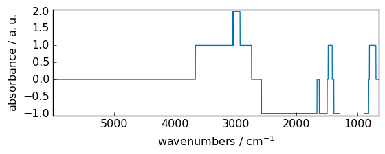
rint

Round elements of the array to the nearest integer, element-wise, keep units

out = np.rint(dataset)
_ = out.plot(figsize=(6, 2.5))  # not that title is not modified for this ufunc

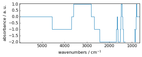
floor

Return the floor of the input, element-wise.

out = np.floor(dataset)
_ = out.plot(figsize=(6, 2.5))

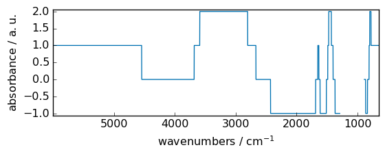
ceil

Return the ceiling of the input, element-wise.

out = np.ceil(dataset)
_ = out.plot(figsize=(6, 2.5))

trunc

Return the truncated value of the input, element-wise.

out = np.trunc(dataset)
_ = out.plot(figsize=(6, 2.5))

Functions affecting magnitudes of the number but also units

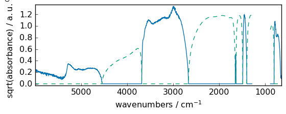
sqrt

Return the non-negative square-root of an array, element-wise.

out = np.sqrt(
    dataset
)  # as they are some negative elements, return dataset has complex dtype.
_ = out.plot_1D(show_complex=True, figsize=(6, 2.5))

 WARNING | (UserWarning) Given trait value dtype "float64" does not match required type "float64". A coerced copy has been created.

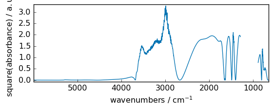
square

Return the element-wise square of the input.

out = np.square(dataset)
_ = out.plot(figsize=(6, 2.5))

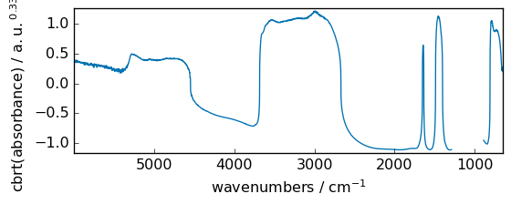
cbrt

Return the cube-root of an array, element-wise.

out = np.cbrt(dataset)
_ = out.plot(figsize=(6, 2.5))

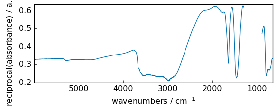
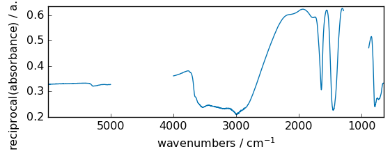
reciprocal

Return the reciprocal of the argument, element-wise.

out = np.reciprocal(dataset + 3.0)
_ = out.plot(figsize=(6, 2.5))

Functions that require no units or dimensionless units for inputs. Returns dimensionless objects.

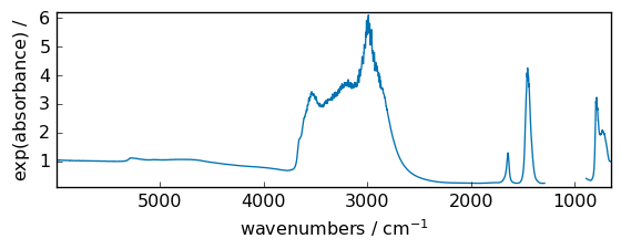
exp

Exponential of all elements in the input array, element-wise

out = np.exp(dataset)
_ = out.plot(figsize=(6, 2.5))

Obviously numpy exponential functions applies only to dimensionless array. Else an error is generated.

x = scp.NDDataset(np.arange(5), units="m")
try:
    np.exp(x)  # A dimensionality error will be generated
except DimensionalityError as e:
    error_(DimensionalityError, e)

 ERROR | DimensionalityError: Cannot convert from 'm' to ''
Function `exp` requires DIMENSIONLESS input

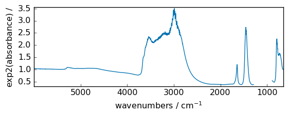
exp2

Calculate 2**p for all p in the input array.

out = np.exp2(dataset)
_ = out.plot(figsize=(6, 2.5))

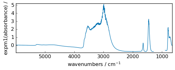
expm1

Calculate exp(x) - 1 for all elements in the array.

out = np.expm1(dataset)
_ = out.plot(figsize=(6, 2.5))

log

Natural logarithm, element-wise.

This doesn’t generate un error for negative numbrs, but the output is masked for those values

out = np.log(dataset)
ax = out.plot(figsize=(6, 2.5), show_mask=True)

 WARNING | (UserWarning) Given trait value dtype "float64" does not match required type "float64". A coerced copy has been created.

out = np.log(dataset - dataset.min())
_ = out.plot(figsize=(6, 2.5))

 WARNING | (UserWarning) Given trait value dtype "float64" does not match required type "float64". A coerced copy has been created.

log2

Base-2 logarithm of x.

out = np.log2(dataset)
_ = out.plot(figsize=(6, 2.5))

 WARNING | (UserWarning) Given trait value dtype "float64" does not match required type "float64". A coerced copy has been created.

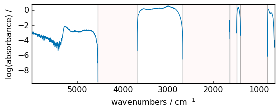
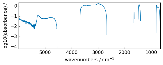
log10

Return the base 10 logarithm of the input array, element-wise.

out = np.log10(dataset)
_ = out.plot(figsize=(6, 2.5))

 WARNING | (UserWarning) Given trait value dtype "float64" does not match required type "float64". A coerced copy has been created.

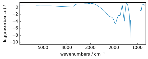
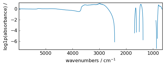
log1p

Return log(x + 1) , element-wise.

out = np.log1p(dataset)
_ = out.plot(figsize=(6, 2.5))

 WARNING | (UserWarning) Given trait value dtype "float64" does not match required type "float64". A coerced copy has been created.

Functions that return numpy arrays (Work only for NDDataset)

sign

Returns an element-wise indication of the sign of a number. Returned object is a ndarray

np.sign(dataset)

masked_array(data=[       1,        1, ...,        1,        1],
             mask=[  False,   False, ...,   False,   False],
       fill_value=1e+20)

np.logical_not(dataset < 0)

masked_array(data=[       1,        1, ...,        1,        1],
             mask=[  False,   False, ...,   False,   False],
       fill_value=True)

isfinite

Test element-wise for finiteness.

np.isfinite(dataset)

masked_array(data=[       1,        1, ...,        1,        1],
             mask=[  False,   False, ...,   False,   False],
       fill_value=True)

isinf

Test element-wise for positive or negative infinity.

np.isinf(dataset)

masked_array(data=[       0,        0, ...,        0,        0],
             mask=[  False,   False, ...,   False,   False],
       fill_value=True)

isnan

Test element-wise for NaN and return result as a boolean array.

np.isnan(dataset)

masked_array(data=[       0,        0, ...,        0,        0],
             mask=[  False,   False, ...,   False,   False],
       fill_value=True)

signbit

Returns element-wise True where signbit is set.

np.signbit(dataset)

masked_array(data=[       0,        0, ...,        0,        0],
             mask=[  False,   False, ...,   False,   False],
       fill_value=True)

Trigonometric functions. Require dimensionless/unitless dataset or radians.

In the below examples, unit of data in dataset is absorbance (then dimensionless)

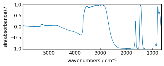
sin

Trigonometric sine, element-wise.

out = np.sin(dataset)
_ = out.plot(figsize=(6, 2.5))

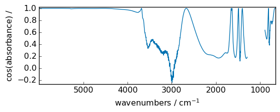
cos

Trigonometric cosine element-wise.

out = np.cos(dataset)
_ = out.plot(figsize=(6, 2.5))

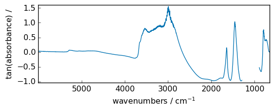
tan

Compute tangent element-wise.

out = np.tan(dataset / np.max(dataset))
_ = out.plot(figsize=(6, 2.5))

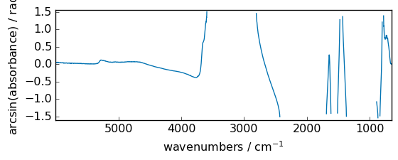
arcsin

Inverse sine, element-wise.

out = np.arcsin(dataset)
_ = out.plot(figsize=(6, 2.5))

 WARNING | (RuntimeWarning) invalid value encountered in arcsin

 WARNING | (UserWarning) Given trait value dtype "float64" does not match required type "float64". A coerced copy has been created.

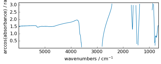
arccos

Trigonometric inverse cosine, element-wise.

out = np.arccos(dataset)
_ = out.plot(figsize=(6, 2.5))

 WARNING | (RuntimeWarning) invalid value encountered in arccos

 WARNING | (UserWarning) Given trait value dtype "float64" does not match required type "float64". A coerced copy has been created.

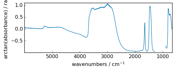
arctan

Trigonometric inverse tangent, element-wise.

out = np.arctan(dataset)
_ = out.plot(figsize=(6, 2.5))

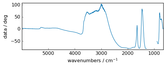
Angle units conversion

rad2deg

Convert angles from radians to degrees (warning: unitless or dimensionless are assumed to be radians, so no error will be issued).

for instance, if we take the z axis (the data magnitude) in the figure above, it’s expressed in radians. We can change to degrees easily.

out = np.rad2deg(dataset)
out.title = "data"  # just to avoid a too long title
_ = out.plot(figsize=(6, 2.5))

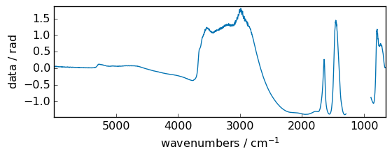
deg2rad

Convert angles from degrees to radians.

out = np.deg2rad(out)
out.title = "data"
_ = out.plot(figsize=(6, 2.5))

Hyperbolic functions

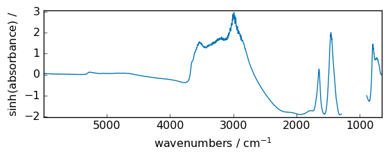
sinh

Hyperbolic sine, element-wise.

out = np.sinh(dataset)
_ = out.plot(figsize=(6, 2.5))

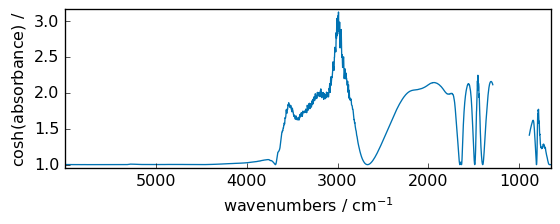
cosh

Hyperbolic cosine, element-wise.

out = np.cosh(dataset)
_ = out.plot(figsize=(6, 2.5))

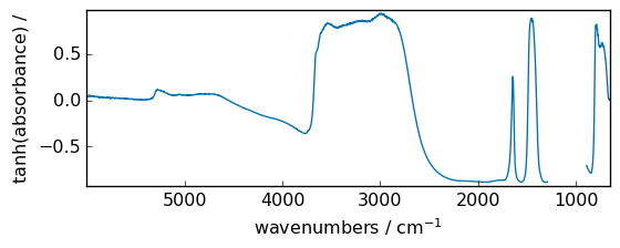
tanh

Compute hyperbolic tangent element-wise.

out = np.tanh(dataset)
_ = out.plot(figsize=(6, 2.5))

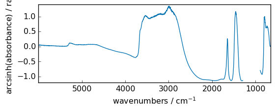
arcsinh

Inverse hyperbolic sine element-wise.

out = np.arcsinh(dataset)
_ = out.plot(figsize=(6, 2.5))

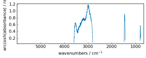
arccosh

Inverse hyperbolic cosine, element-wise.

out = np.arccosh(dataset)
_ = out.plot(figsize=(6, 2.5))

 WARNING | (UserWarning) Given trait value dtype "float64" does not match required type "float64". A coerced copy has been created.

arctanh

Inverse hyperbolic tangent element-wise.

out = np.arctanh(dataset)
_ = out.plot(figsize=(6, 2.5))

 WARNING | (RuntimeWarning) invalid value encountered in arctanh

 WARNING | (UserWarning) Given trait value dtype "float64" does not match required type "float64". A coerced copy has been created.

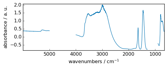
Binary functions

dataset2 = np.reciprocal(dataset + 3)  # create a second dataset
dataset2[5000.0:4000.0] = MASKED
_ = dataset.plot(figsize=(6, 2.5))
_ = dataset2.plot(figsize=(6, 2.5))

Arithmetic

add

Add arguments element-wise.

out = np.add(dataset, dataset2)
_ = out.plot(figsize=(6, 2.5))

subtract

Subtract arguments, element-wise.

out = np.subtract(dataset, dataset2)
_ = out.plot(figsize=(6, 2.5))

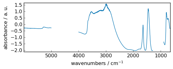
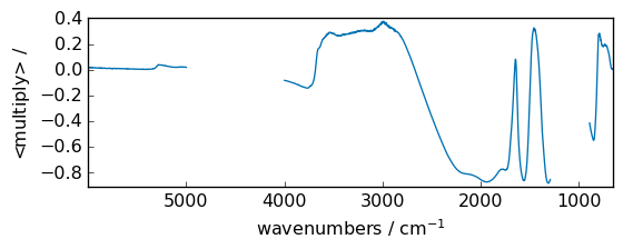
multiply

Multiply arguments element-wise.

out = np.multiply(dataset, dataset2)
_ = out.plot(figsize=(6, 2.5))

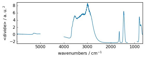
divide

or ##### true_divide Returns a true division of the inputs, element-wise.

out = np.divide(dataset, dataset2)
_ = out.plot(figsize=(6, 2.5))

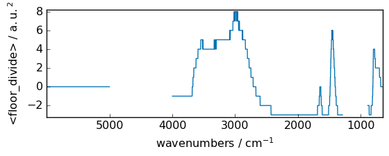
floor_divide

Return the largest integer smaller or equal to the division of the inputs.

out = np.floor_divide(dataset, dataset2)
_ = out.plot(figsize=(6, 2.5))

Complex or hypercomplex NDDatasets

NDDataset objects with complex data are handled differently than in numpy.ndarray .

Instead, complex data are stored by interlacing the real and imaginary part. This allows the definition of data that can be complex in several axis, and e .g., allows 2D-hypercomplex array that can be transposed (useful for NMR data).

da = scp.NDDataset(
    [
        [1.0 + 2.0j, 2.0 + 0j],
        [1.3 + 2.0j, 2.0 + 0.5j],
        [1.0 + 4.2j, 2.0 + 3j],
        [5.0 + 4.2j, 2.0 + 3j],
    ]
)
da

name	NDDataset_532fc138
author	runner@fv-az1501-19
created	2024-04-28 03:12:04+02:00
DATA
title
values	R[[ 1 2] [ 1.3 2] [ 1 2] [ 5 2]] I[[ 2 0] [ 2 0.5] [ 4.2 3] [ 4.2 3]]
shape	(y:4, x:2(complex))

A dataset of type float can be transformed into a complex dataset (using two consecutive rows to create a complex row)

da = scp.NDDataset(np.arange(40).reshape(10, 4))
da

name	NDDataset_53310afc
author	runner@fv-az1501-19
created	2024-04-28 03:12:04+02:00
DATA
title
values	[[ 0 1 2 3] [ 4 5 6 7] ... [ 32 33 34 35] [ 36 37 38 39]]
shape	(y:10, x:4)

dac = da.set_complex()
dac

name	NDDataset_5331ffac
author	runner@fv-az1501-19
created	2024-04-28 03:12:04+02:00
DATA
title
values	R[[ 0 2] [ 4 6] ... [ 32 34] [ 36 38]] I[[ 1 3] [ 5 7] ... [ 33 35] [ 37 39]]
shape	(y:10, x:2(complex))

Note the xdimension size is divided by a factor of two

A dataset which is complex in two dimensions is called hypercomplex (it’s datatype in SpectroChemPy is set to quaternion).

daq = da.set_quaternion()  # equivalently one can use the set_hypercomplex method
daq

name	NDDataset_53334e84
author	runner@fv-az1501-19
created	2024-04-28 03:12:04+02:00
DATA
title
values	RR[[ 0 2] [ 8 10] ... [ 24 26] [ 32 34]] RI[[ 1 3] [ 9 11] ... [ 25 27] [ 33 35]] IR[[ 4 6] [ 12 14] ... [ 28 30] [ 36 38]] II[[ 5 7] [ 13 15] ... [ 29 31] [ 37 39]]
shape	(y:5(complex), x:2(complex))

daq.dtype

dtype(quaternion)