MCR ALS
[1]:
import spectrochempy as scp

|
SpectroChemPy's API - v.0.6.9.dev9 © Copyright 2014-2024 - A.Travert & C.Fernandez @ LCS |
Introduction
MCR-ALS (standing for Multivariate Curve Resolution - Alternating Least Squares) is a popular method for resolving a set (or several sets) of spectra \(X\) of an evolving mixture (or a set of mixtures) into the spectra \(S^t\) of ‘pure’ species and their concentration profiles \(C\). In terms of matrix equation:
The ALS algorithm allows applying soft or hard constraints (e.g., non negativity, unimodality, equality to a given profile) to the spectra or concentration profiles of pure species. This property makes MCR-ALS an extremely flexible and powerful method.
In this tutorial, the application of MCS-ALS as implemented in Scpy to a ‘classical’ dataset form the literature is presented.
The (minimal) dataset
Here, we perform the MCR ALS optimization of a dataset corresponding to a HPLC-DAD run, from Jaumot et al. Chemolab, 76 (2005), pp. 101-110 and Jaumot et al. Chemolab, 140 (2015) pp. 1-12. This dataset (and others) can be loaded from the “Multivariate Curve Resolution Homepage” at https://mcrals.wordpress.com/download/example-data-sets. For the user convenience, this dataset is present in the ‘datadir’ of spectrochempy in ‘als2004dataset.MAT’ and can be read as follows in Scpy:
[2]:
A = scp.read_matlab("matlabdata/als2004dataset.MAT")
The .mat file contains 6 matrices which are thus returned in A as a list of 6 NDDatasets. We print the names and dimensions of these datasets:
[3]:
for a in A:
    print(f"{a.name} : {a.shape}")
cpure : (204, 4)
MATRIX : (204, 96)
isp_matrix : (4, 4)
spure : (4, 96)
csel_matrix : (51, 4)
m1 : (51, 96)
In this tutorial, we are first interested in the dataset named (‘m1’) that contains a singleHPLC-DAD run(s). As usual, the rows correspond to the ‘time axis’ of the HPLC run(s), and the columns to the ‘wavelength’ axis of the UV spectra.
Let’s name it ‘X’ (as in the matrix equation above), display its content and plot it:
[4]:
X = A[-1]
X
[4]:
| name | m1 |
| author | runner@fv-az1501-19 |
| created | 2024-04-28 03:09:36+02:00 |
| history | 2024-04-28 03:09:36+02:00> Imported from .mat file |
| DATA | |
| title | |
| values | [[ 0.01525 0.01285 ... 0.0003178 -0.0002631] [ 0.01969 0.01617 ... -0.007001 0.000682] ... [ 0.01 0.0144 ... -0.0007125 0.004296] [0.008121 0.01139 ... -0.007331 -0.001341]] |
| shape | (y:51, x:96) |
[5]:
_ = X.plot()
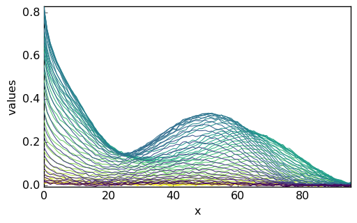
The original dataset is the ‘m1’ matrix and does not contain information as to the actual elution time, wavelength, and data units. Hence, the resulting NDDataset has no coordinates and on the plot, only the matrix line and row indexes are indicated. For the clarity of the tutorial, we add: (i) a proper title to the data, (ii) the default coordinates (index) do the NDDataset and (iii) a proper name for these coordinates:
[6]:
X.title = "absorbance"
X.set_coordset(None, None)
X.set_coordtitles(y="elution time", x="wavelength")
X
[6]:
| name | m1 |
| author | runner@fv-az1501-19 |
| created | 2024-04-28 03:09:36+02:00 |
| history | 2024-04-28 03:09:36+02:00> Imported from .mat file |
| DATA | |
| title | absorbance |
| values | [[ 0.01525 0.01285 ... 0.0003178 -0.0002631] [ 0.01969 0.01617 ... -0.007001 0.000682] ... [ 0.01 0.0144 ... -0.0007125 0.004296] [0.008121 0.01139 ... -0.007331 -0.001341]] |
| shape | (y:51, x:96) |
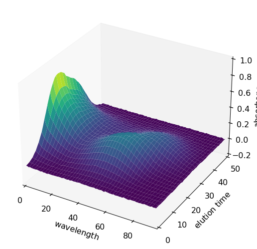
From now on, these names will be taken into account by Scpy in the plots as well as in the analysis treatments (PCA, EFA, MCR-ALs, …). For instance to plot X as a surface:
[7]:
surf = X.plot_surface(linewidth=0.0, figsize=(10, 5), autolayout=False)
Initial guess and MCR ALS optimization
The ALS optimization of the MCR equation above requires the input of a guess for either the concentration matrix \(C_0\) or the spectra matrix \(S^t_0\). Given the data matrix \(X\), the lacking initial matrix (\(S^t_0\) or \(C_0\), respectively) is computed by:
or
Case of initial spectral profiles
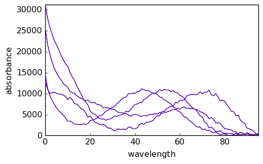
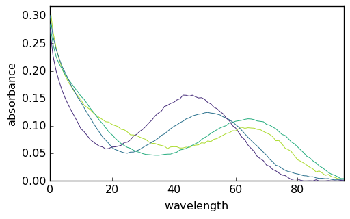
The matrix spure provided in the initial dataset is a guess for the spectral profiles. Let’s name it ‘St0’, and plot it:
[8]:
St0 = A[3]
_ = St0.plot()
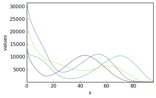
Note that, again, no information has been given as to the ordinate and abscissa data. We could add them as previously but this is not very important. The key point is that the ‘wavelength’ dimension is compatible with the data ‘X’, which is indeed the case (both have a length of 95). If it was not, an error would be generated in the following.
ALS Optimization
With this guess ‘St0’ and the dataset ‘X’ we can create a MCRALS object. At this point of the tutorial, we will use all the default parameters.
First, we create an instance of a MCRALS object:
[9]:
mcr = scp.MCRALS(log_level="INFO")
The fit method of mcr is now used to start the iteration process. As the log level has been set to “INFO” at the MCRALS instance creation, so we have a summary of the ALS iterations
[10]:
mcr.fit(X, St0)
Spectra profile initialized with 4 components
Initial concentration profile computed
*** ALS optimisation log ***
#iter RSE / PCA RSE / Exp %change
-------------------------------------------------
1 0.000442 0.002807 -97.747926
2 0.000433 0.002805 -0.048763
converged !
[10]:
<spectrochempy.analysis.decomposition.mcrals.MCRALS at 0x7f16287278b0>
The optimization has converged within few iterations. The figures reported for each iteration are defined as follows:
‘Error/PCA’ is the standard deviation of the residuals with respect to data reconstructed by a PCA with as many components as pure species (4 in this example),
‘Error/exp’: is the standard deviation of the residuals with respect to the experimental data X,
‘%change’: is the percent change of ‘Error/exp’ between 2 iterations
The default is to stop when this %change between two iteration is negative (so that the solution is improving), but with an absolute value lower than 0.1% (so that the improvement is considered negligible). This parameter - as well as several other parameters affecting the ALS optimization can be changed by the setting the ‘tol’ value. For instance:
[11]:
mcr.tol = 0.01
mcr.fit(X, St0)
*** ALS optimisation log ***
#iter RSE / PCA RSE / Exp %change
-------------------------------------------------
1 0.000442 0.002807 -97.747926
2 0.000433 0.002805 -0.048763
3 0.000429 0.002805 -0.022012
4 0.000428 0.002804 -0.008682
converged !
[11]:
<spectrochempy.analysis.decomposition.mcrals.MCRALS at 0x7f16287278b0>
As could be expected more iterations have been necessary to reach this stricter convergence criterion. The other convergence criterion that can be fixed by the user is ‘maxdiv’, the maximum number of successive diverging iterations. It is set to 5 by default and allows for stopping the ALS algorithm when it is no converging. If for instance the ‘tol’ is set very low, the optimization will be stopped when either the maximum number of iterations is reached (max_iter, 50 by default) or when no improvement is during 5 successive iterations (maxdiv).
[12]:
mcr.tol = 0.001
mcr.fit(X, St0)
*** ALS optimisation log ***
#iter RSE / PCA RSE / Exp %change
-------------------------------------------------
1 0.000442 0.002807 -97.747926
2 0.000433 0.002805 -0.048763
3 0.000429 0.002805 -0.022012
4 0.000428 0.002804 -0.008682
5 0.000427 0.002804 -0.003700
6 0.000427 0.002804 -0.000845
converged !
[12]:
<spectrochempy.analysis.decomposition.mcrals.MCRALS at 0x7f16287278b0>
More information about the MCRALS estimator
To get help about the different configuration parameters
[13]:
# help(mcr)
[14]:
# It is possible to chain fit runs, without recomputing everything for example for
# optimization of some parameters

mcr = scp.MCRALS(tol=0.001, log_level="INFO")
_ = mcr.fit(X, St0)
Spectra profile initialized with 4 components
Initial concentration profile computed
*** ALS optimisation log ***
#iter RSE / PCA RSE / Exp %change
-------------------------------------------------
1 0.000442 0.002807 -97.747926
2 0.000433 0.002805 -0.048763
3 0.000429 0.002805 -0.022012
4 0.000428 0.002804 -0.008682
5 0.000427 0.002804 -0.003700
6 0.000427 0.002804 -0.000845
converged !
[15]:
mcr1 = scp.MCRALS(tol=0.1, log_level="INFO")
_ = mcr1.fit(X, St0)
Spectra profile initialized with 4 components
Initial concentration profile computed
*** ALS optimisation log ***
#iter RSE / PCA RSE / Exp %change
-------------------------------------------------
1 0.000442 0.002807 -97.747926
2 0.000433 0.002805 -0.048763
converged !
[16]:
mcr1.tol = 0.01
_ = mcr1.fit(
    X, (mcr1.C.copy(), mcr1.St.copy())
)  # reuse C and ST computed at the previous run
print("second run with the output of the first")
*** ALS optimisation log ***
#iter RSE / PCA RSE / Exp %change
-------------------------------------------------
1 0.000429 0.002805 -97.749519
2 0.000428 0.002804 -0.008682
converged !
second run with the output of the first
[17]:
mcr1.tol = 0.001
_ = mcr1.fit(X, (mcr1.C, mcr1.St))
print("third run with the output of the second")
*** ALS optimisation log ***
#iter RSE / PCA RSE / Exp %change
-------------------------------------------------
1 0.000427 0.002804 -97.749798
2 0.000427 0.002804 -0.000845
converged !
third run with the output of the second
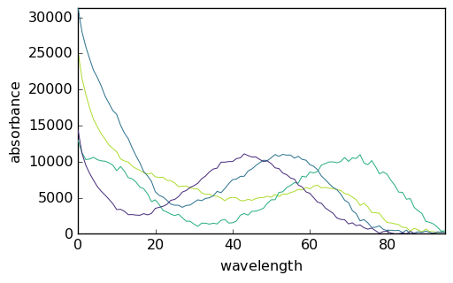
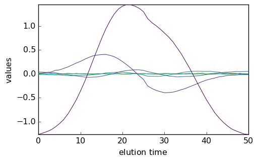
Below we compare the outputs of the initial run (red) and final run (blue).
[18]:
_ = mcr.C.T.plot(cmap=None, color="red")
_ = mcr1.C.T.plot(clear=False, cmap=None, color="blue")

_ = mcr.St.plot(cmap=None, color="red")
_ = mcr1.St.plot(clear=False, cmap=None, color="blue")
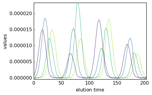
Solutions
The solutions of the MCR ALS optimization are the optimized concentration (C) and pure spectra (St) datasets. They are stored as in the C and St attribute of the MCRAL object. As MCRALS is derived from to the DecompositionAnalysis class, C and St can also be obtained by MCRALS.transform() and MCRALS.components, respectively.
Let’s generate a MCRALS object with the default settings, and get the solution datasets C and St. Note that the default log_level is “WARNING” so we do not see any output here.
[19]:
mcr1 = scp.MCRALS()
mcr1.fit(X, St0)
[19]:
<spectrochempy.analysis.decomposition.mcrals.MCRALS at 0x7f162846d180>
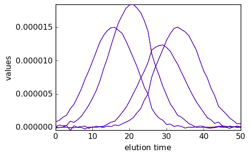
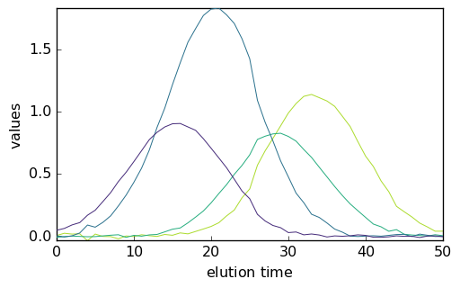
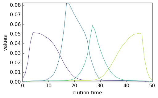
As the dimensions of C are such that the rows’ direction (C.y) corresponds to the elution time and the columns’ direction (C.x) correspond to the four pure species, it is necessary to transpose it before plotting in order to plot the concentration vs. the elution time.
[20]:
_ = mcr1.C.T.plot()

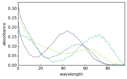
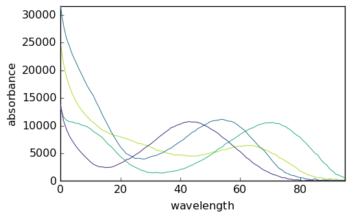
On the other hand, the spectra of the pure species can be plotted directly:
[21]:
_ = mcr1.St.plot()
A basic illustration of the rotational ambiguity
We have thus obtained the elution profiles of the four pure species. Note that the ‘concentration’ values are very low. This results from the fact that the absorbance values in X are on the order of 0-1 while the absorbance of the initial pure spectra are of the order of 10^4. As can be seen above, the absorbance of the final spectra is of the same order of magnitude.
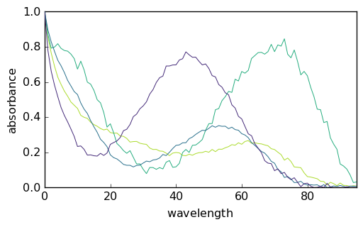
It is possible to normalize the intensity of the spectral profiles by setting the ‘normSpec’ parameter to True. With this option, the spectra are normalized such that their euclidean norm is 1. The other normalization option is normspec = ‘max’, whereby the maximum intensity of the spectra is 1. Let’s look at the effect of both normalizations:
[22]:
mcr2 = scp.MCRALS(normSpec="euclid")
mcr2.fit(X, St0)

mcr3 = scp.MCRALS(normSpec="max")
mcr3.fit(X, St0)

_ = mcr1.St.plot()
_ = mcr2.St.plot()
_ = mcr3.St.plot()

[23]:
_ = mcr1.C.T.plot()
_ = mcr2.C.T.plot()
_ = mcr3.C.T.plot()

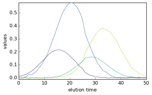
It is clear that the normalization affects the relative intensity of the spectra and of the concentration. This is a basic example of the well known rotational ambiguity of the MCS ALS solutions.
Guessing the concentration profile with PCA + EFA
Generally, in MCR ALS, the initial guess cannot be obtained independently of the experimental data ‘x’. In such a case, one has to rely on ‘X’ to obtained (i) the number of pure species and (ii) their initial concentrations or spectral profiles. The number of pure species can be assessed by carrying out a PCA on the data while the concentrations or spectral profiles can be estimated using procedures such EFA of SIMPLISMA. The following will illustrate the use of PCA followed by EFA
Use of PCA to assess the number of pure species
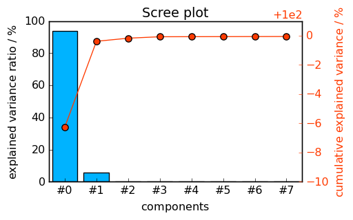
Let’s first analyse our dataset using PCA and plot a screeplot:
[24]:
pca = scp.PCA(n_components=8)
pca.fit(X)
pca.printev()
_ = pca.screeplot()
PC      Eigenvalue              %variance               %cumulative
         of cov(X)                 per PC                  variance
#1       9.775e-01                 93.740                    93.740
#2       2.447e-01                  5.875                    99.614
#3       4.659e-02                  0.213                    99.827
#4       3.176e-02                  0.099                    99.926
#5       6.673e-03                  0.004                    99.931
#6       6.587e-03                  0.004                    99.935
#7       6.382e-03                  0.004                    99.939
#8       6.134e-03                  0.004                    99.943
<Figure size 528x336 with 0 Axes>
The number of significant PC’s is clearly larger or equal to 2. It is, however, difficult to determine whether it should be set to 3 or 4… Let’s look at the score and loading matrices:
[25]:
scores = pca.transform()
_ = pca.loadings.plot()
_ = scores.T.plot()
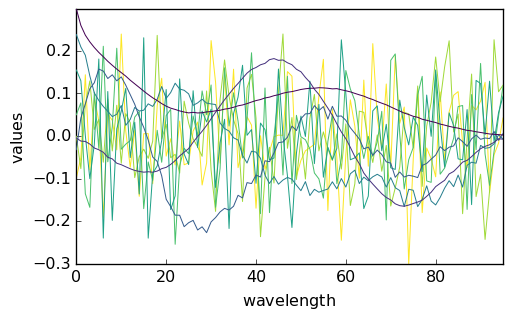
Examination of the scores and loadings indicate that the 4th component has structured, nonrandom scores and loadings. Hence, we will fix the number of pure species to 4.
Determination of initial concentrations using EFA
Once the number of components has been determined, the initial concentration matrix is obtained very easily using EFA:
[26]:
efa = scp.EFA()
efa.fit(X)
efa.n_components = 4
C0 = efa.transform()
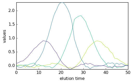
_ = C0.T.plot()
The MCR ALS can then be launched using this new guess:
[27]:
mcr4 = scp.MCRALS(max_iter=100, normSpec="euclid")
mcr4.fit(X, C0)
[27]:
<spectrochempy.analysis.decomposition.mcrals.MCRALS at 0x7f162826b940>
[28]:
_ = mcr4.C.T.plot()
_ = mcr4.St.plot()
Augmented datasets
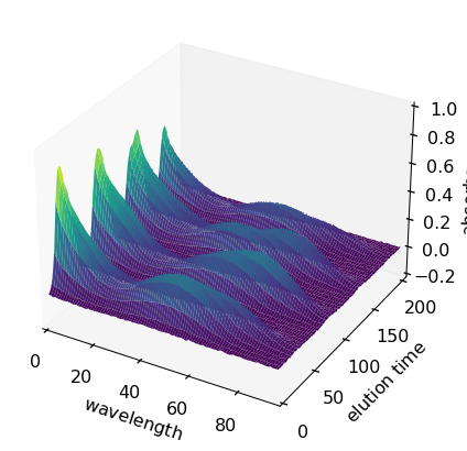
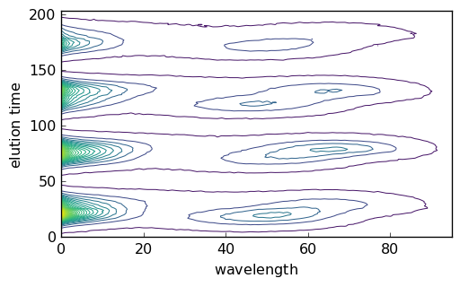
The ‘MATRIX’ dataset is a columnwise augmented dataset consisting into 5 successive runs:
[29]:
A[1]
[29]:
| name | MATRIX |
| author | runner@fv-az1501-19 |
| created | 2024-04-28 03:09:36+02:00 |
| history | 2024-04-28 03:09:36+02:00> Imported from .mat file |
| DATA | |
| title | |
| values | [[ 0.01525 0.01285 ... 0.0003178 -0.0002631] [ 0.01969 0.01617 ... -0.007001 0.000682] ... [0.005205 0.003604 ... 0.0001341 0.004421] [0.001699 0.007194 ... -2.012e-05 0.003973]] |
| shape | (y:204, x:96) |
Let’s plot it as a surface and as a map:
[30]:
X2 = A[1]
X2.title = "absorbance"
X2.set_coordset(None, None)
X2.set_coordtitles(y="elution time", x="wavelength")
surf = X2.plot_surface(linewidth=0.0, ccount=100, figsize=(8, 4), autolayout=False)
_ = X2.plot(method="map")
[31]:
mcr5 = scp.MCRALS(unimodConc=[])
mcr5.fit(X2, St0)
[31]:
<spectrochempy.analysis.decomposition.mcrals.MCRALS at 0x7f1629b18ee0>
[32]:
_ = mcr5.C.T.plot()
[33]:
_ = mcr5.St.plot()
[To be continued…]