Baseline corrections

This tutorial shows how to make baseline corrections with spectrochempy. As prerequisite, the user is expected to have read the Import and Import IR tutorials.

import spectrochempy as scp

SpectroChemPy's API - v.0.6.5 © Copyright 2014-2023 - A.Travert & C.Fernandez @ LCS

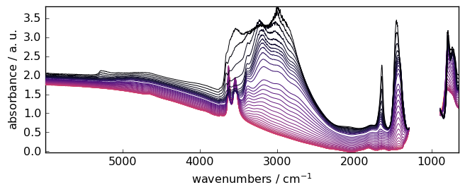
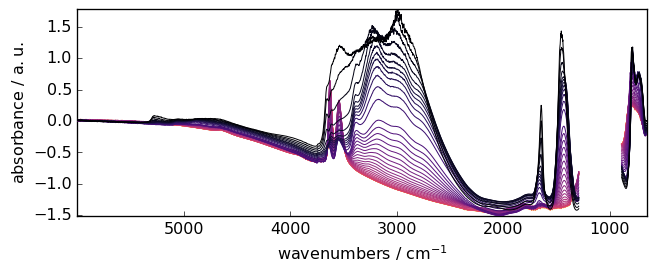
Now let’s import and plot a typical IR dataset which was recorded during the removal of ammonia from a NH4-Y zeolite:

X = scp.read_omnic("irdata/nh4y-activation.spg")
X[:, 1290.0:890.0] = scp.MASKED

After setting some plotting preferences and plot it

prefs = X.preferences
prefs.figure.figsize = (7, 3)
prefs.colormap = "magma"
_ = X.plot()

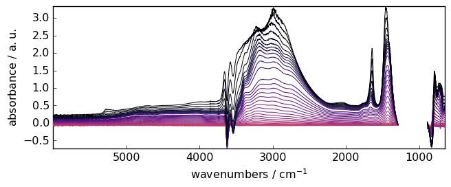
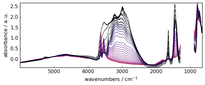
Background subtraction

Often, particularly for surface species, the baseline is first corrected by subtracting a reference spectrum. In this example, it could be, for instance, the last spectrum (index -1). Hence:

Xdiff = X - X[-1]
_ = Xdiff.plot()

Detrend

Other simple baseline corrections - often use in preprocessing prior chemometric analysis - constist in shifting the spectra or removing a linear trend. This is done using the detrend() method, which is a wrapper of the [ detrend() method] (https://docs.scipy.org/doc/scipy/reference/generated/scipy.signal.detrend.html) from the scipy.signal module to which we refer the interested reader.

Linear trend

Subtract the linear trend of each spectrum (type=’linear’, default)

_ = X.detrend().plot()

Constant trend

Subtract the average absorbance to each spectrum

_ = X.detrend(type="constant").plot()

Automatic linear baseline correction abc

When the baseline to remove is a simple linear correction, one can use abc . This performs an automatic baseline correction.

_ = scp.abc(X).plot()

Advanced baseline correction

‘Advanced’ baseline correction basically consists for the user to choose:

• spectral ranges which s/he considers as belonging to the baseline - the type of polynomial(s) used to model the baseline in and between these regions (keyword: interpolation ) - the method used to apply the correction to spectra: sequentially to each spectrum, or using a multivariate approach (keyword: method ).

Range selection

Each spectral range is defined by a list of two values indicating the limits of the spectral ranges, e.g. [4500., 3500.] to select the 4500-3500 cm\(^{-1}\) range. Note that the ordering has no importance and using [3500.0, 4500.] would lead to exactly the same result. It is also possible to formally pick a single wavenumber 3750. .

The first step is then to select the various regions that we expect to belong to the baseline

ranges = [5900.0, 5400.0], 4550.0, [4500.0, 4000.0], [2100.0, 2000.0], [1550.0, 1555.0]

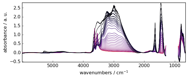
After selection of the baseline ranges, the baseline correction can be made using a sequence of 2 commands:

1. Initialize an instance of BaselineCorrection

blc = scp.BaselineCorrection(X)

2. compute baseline other the ranges

Xcorr = blc.compute(ranges)
Xcorr

name	nh4y-activation
author	runner@fv-az626-878
created	2023-06-06 01:31:00+00:00
history	2023-06-06 01:30:57+00:00> Imported from spg file /home/runner/.spectrochempy/testdata/irdata/nh4y-activation.spg. 2023-06-06 01:30:57+00:00> Sorted by date 2023-06-06 01:31:00+00:00> Baseline correction. Method: 2023-06-06 01:31:00+00:00> Sequential. 2023-06-06 01:31:00+00:00> Interpolation: Polynomial, order=1.
DATA
title	absorbance
values	[[ -0.1746 -0.1708 ... 1.433 1.432] [ -0.1709 -0.1666 ... 1.382 1.382] ... [ -0.1653 -0.1671 ... 1.53 1.53] [ -0.1674 -0.1675 ... 1.546 1.544]] a.u.
shape	(y:55, x:5549)
DIMENSION `x`
size	5549
title	wavenumbers
coordinates	[ 6000 5999 ... 650.9 649.9] cm⁻¹
DIMENSION `y`
size	55
title	acquisition timestamp (GMT)
coordinates	[1.468e+09 1.468e+09 ... 1.468e+09 1.468e+09] s
labels	[[ 2016-07-06 19:03:14+00:00 2016-07-06 19:13:14+00:00 ... 2016-07-07 04:03:17+00:00 2016-07-07 04:13:17+00:00] [ vz0466.spa, Wed Jul 06 21:00:38 2016 (GMT+02:00) vz0467.spa, Wed Jul 06 21:10:38 2016 (GMT+02:00) ... vz0520.spa, Thu Jul 07 06:00:41 2016 (GMT+02:00) vz0521.spa, Thu Jul 07 06:10:41 2016 (GMT+02:00)]]

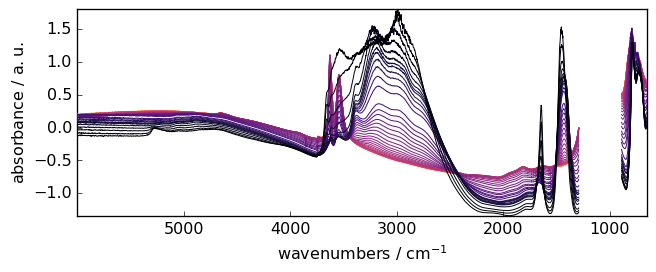
• plot the result (blc.corrected.plot() would lead to the same result)

_ = Xcorr.plot()

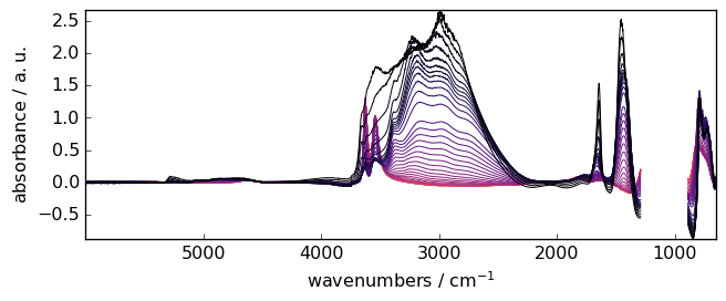
Interpolation method

The previous correction was made using the default parameters for the interpolation ,i.e. an interpolation using cubic Hermite spline interpolation: interpolation='pchip' (pchip stands for Piecewise Cubic Hermite Interpolating Polynomial). This option triggers the use of scipy.interpolate.PchipInterpolator() to which we refer the interested readers. The other interpolation method is the classical polynomial interpolation (interpolation='polynomial' ) in which case the order can also be set (e.g. order=3 , the default value being 6). In this case, the base methods used for the interpolation are those of the polynomial module of spectrochempy, in particular the polyfit() method.

For instance:

First, we put the ranges in a list

ranges = [[5900.0, 5400.0], [4000.0, 4500.0], [2100.0, 2000.0], [1550.0, 1555.0]]

Warning

if you use a tuple to define the sequences of ranges:

ranges = [5900.0, 5400.0], [4000., 4500.], [2100., 2000.0], [1550., 1555.]

or

ranges = ([5900.0, 5400.0], [4000., 4500.], [2100., 2000.0], [1550., 1555.])

then you can call compute by directly pass the ranges tuple, or you can unpack it as below.

blc.compute(ranges, ....)

if you use a list instead of tuples:

ranges = [[5900.0, 5400.0], [4000., 4500.], [2100., 2000.0], [1550., 1555.]]

then you MUST UNPACK the element when calling compute:

blc.compute(*ranges, ....)

blc = scp.BaselineCorrection(X)
blc.compute(*ranges, interpolation="polynomial", order=6)

name	nh4y-activation
author	runner@fv-az626-878
created	2023-06-06 01:31:00+00:00
history	2023-06-06 01:30:57+00:00> Imported from spg file /home/runner/.spectrochempy/testdata/irdata/nh4y-activation.spg. 2023-06-06 01:30:57+00:00> Sorted by date 2023-06-06 01:31:01+00:00> Baseline correction. Method: 2023-06-06 01:31:01+00:00> Sequential. 2023-06-06 01:31:01+00:00> Interpolation: Polynomial, order=6.
DATA
title	absorbance
values	[[-0.02411 -0.02017 ... 0.001605 -0.00293] [-0.03628 -0.03177 ... 0.001021 -0.003108] ... [-0.01756 -0.01955 ... -0.0004106 -0.003214] [-0.02053 -0.02076 ... 0.00117 -0.003751]] a.u.
shape	(y:55, x:5549)
DIMENSION `x`
size	5549
title	wavenumbers
coordinates	[ 6000 5999 ... 650.9 649.9] cm⁻¹
DIMENSION `y`
size	55
title	acquisition timestamp (GMT)
coordinates	[1.468e+09 1.468e+09 ... 1.468e+09 1.468e+09] s
labels	[[ 2016-07-06 19:03:14+00:00 2016-07-06 19:13:14+00:00 ... 2016-07-07 04:03:17+00:00 2016-07-07 04:13:17+00:00] [ vz0466.spa, Wed Jul 06 21:00:38 2016 (GMT+02:00) vz0467.spa, Wed Jul 06 21:10:38 2016 (GMT+02:00) ... vz0520.spa, Thu Jul 07 06:00:41 2016 (GMT+02:00) vz0521.spa, Thu Jul 07 06:10:41 2016 (GMT+02:00)]]

The corrected attribute contains the corrected NDDataset.

_ = blc.corrected.plot()

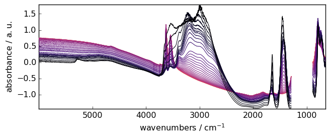
Multivariate method

The method option defines whether the selected baseline regions of the spectra should be taken ‘as is’ this is the default method='sequential' ), or modeled using a multivariate approach (method='multivariate' ).

The 'multivariate' option is useful when the signal‐to‐noise ratio is low and/or when the baseline changes in various regions of the spectrum are correlated. It consist in (i) modeling the baseline regions by a principal component analysis (PCA), (ii) interpolate the loadings of the first principal components over the whole spectral and (iii) modeling the spectra baselines from the product of the PCA scores and the interpolated loadings. (for detail: see Vilmin et al. Analytica Chimica Acta 891 (2015)).

If this option is selected, the user should also choose npc , the number of principal components used to model the baseline. In a sense, this parameter has the same role as the order parameter, except that it will affect how well the baseline fits the selected regions, but on both dimensions: wavelength and acquisition time. In particular a large value of npc will lead to overfit of baseline variation with time and will lead to the same result as the sequential method while a too small value would miss important principal component underlying the baseline change over time. Typical optimum values are npc=2 or npc=3 (see Exercises below).

blc = scp.BaselineCorrection(X)
blc.compute(*ranges, interpolation="pchip", method="multivariate", npc=2)
_ = blc.corrected.plot()

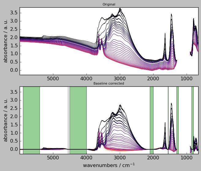
Code snippet for ‘advanced’ baseline correction

The following code in which the user can change any of the parameters and look at the changes after re-running the cell:

# user defined parameters
# -----------------------
ranges = (
    [5900.0, 5400.0],
    [4000.0, 4500.0],
    4550.0,
    [2100.0, 2000.0],
    [1550.0, 1555.0],
    [1250.0, 1300.0],
    [800.0, 850.0],
)
interpolation = "pchip"  # choose 'polynomial' or 'pchip'
order = 5  # only used for 'polynomial'
method = "sequential"  # choose 'sequential' or 'multivariate'
npc = 3  # only used for 'multivariate'

# code: compute baseline, plot original and corrected NDDatasets and ranges
# --------------------------------------------------------------------------------------
blc = scp.BaselineCorrection(X)
Xcorr = blc.compute(
    *ranges, interpolation=interpolation, order=order, method=method, npc=npc
)

axes = scp.multiplot(
    [X, Xcorr],
    labels=["Original", "Baseline corrected"],
    sharex=True,
    nrow=2,
    ncol=1,
    figsize=(7, 6),
    dpi=96,
)
blc.show_regions(axes["axe21"])

Widget for “advanced” baseline corrections

The BaselineCorrector widget can be used in either Jupyter notebook or Jupyter lab.

The buttons are the following: * upload: allows to upload new data. * process : baseline correct and plot original dataset + baseline and corrected datasets * save as: save the baseline corrected dataset.

The x slice and y slice text boxes can be used to slice the original dataset with the usual [start:stop:step] format. In both dimensions, coordinates or indexes can be used (for example, [3000.0::2] or [:100:5] are valid entries).

The Method and Interpolation dropdown fields are self-explanatory, see above for details.

Ranges must be entered as a tuple of digits or wave numbers, e.g. ([5900.0, 5400.0], 2000.0, [1550.0, 1555.0],) .

X = scp.read_omnic("irdata/nh4y-activation.spg")
out = scp.BaselineCorrector(X)

After processing, one can get the original (sliced) dataset, corrected dataset and baselines through the following attributes:

out.original, out.corrected, out.baseline

(NDDataset: [float64] a.u. (shape: (y:55, x:5549)),
 NDDataset: [float64] a.u. (shape: (y:55, x:5549)),
 NDDataset: [float64] a.u. (shape: (y:55, x:5549)))

Exercises

basic: - write commands to subtract (i) the first spectrum from a dataset and (ii) the mean spectrum from a dataset - write a code to correct the baseline of the last 10 spectra of the above dataset in the 4000-3500 cm\(^{-1}\) range

intermediate: - what would be the parameters to use in ‘advanced’ baseline correction to mimic ‘detrend’ ? Write a code to check your answer.

advanced: - simulate noisy spectra with baseline drifts and compare the performances of multivariate vs sequential methods