Apodization
[1]:
import spectrochempy as scp
from spectrochempy.core.units import ur

|
SpectroChemPy's API - v.0.6.9.dev9 © Copyright 2014-2024 - A.Travert & C.Fernandez @ LCS |
Introduction
As an example, apodization is a transformation particularly useful for preprocessing NMR time domain data before Fourier transformation. It generally helps for signal-to-noise improvement.
[2]:
# read an experimental spectra
path = scp.pathclean("nmrdata/bruker/tests/nmr/topspin_1d")

# the method pathclean allow to write pth in linux or window style indifferently
dataset = scp.read_topspin(path, expno=1, remove_digital_filter=True)
dataset = dataset / dataset.max()  # normalization

# store original data
nd = dataset.copy()

# show data
nd
[2]:
| name | topspin_1d expno:1 procno:1 (FID) |
| author | runner@fv-az1106-694 |
| created | 2024-04-27 03:06:10+02:00 |
| history | 2024-04-27 03:06:11+02:00> Binary operation truediv with `(2283.5096153847107-2200.383064516033j) pp` has been performed |
| DATA | |
| title | intensity |
| values | R[ 0.4717 1 ... 3.96e-05 -1.135e-05] I[0.0003036 0 ... 6.533e-05 -3.403e-05] |
| size | 12411 (complex) |
| DIMENSION `x` | |
| size | 12411 |
| title | F1 acquisition time |
| coordinates | [ 0 4 ... 4.964e+04 4.964e+04] µs |
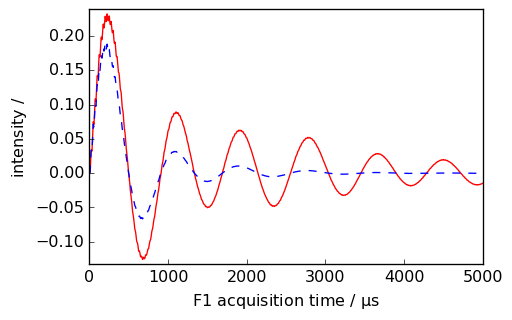
Plot of the Real and Imaginary original data
[3]:
_ = nd.plot(xlim=(0.0, 15000.0))
_ = nd.plot(imag=True, data_only=True, clear=False, color="r")
Exponential multiplication
[4]:
_ = nd.plot(xlim=(0.0, 15000.0))
_ = nd.em(lb=300.0 * ur.Hz)
_ = nd.plot(data_only=True, clear=False, color="g")
Warning: processing function are most of the time applied inplace. Use inplace=False option to avoid this if necessary
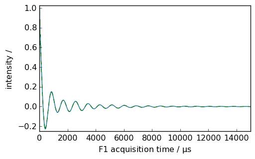
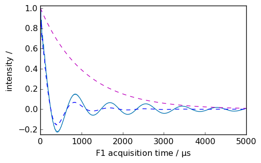
[5]:
nd = dataset.copy()  # to go back to the original data
_ = nd.plot(xlim=(0.0, 5000.0))
ndlb = nd.em(lb=300.0 * ur.Hz, inplace=False)  # ndlb contain the processed data
_ = nd.plot(data_only=True, clear=False, color="g")  # nd dataset remain unchanged
_ = ndlb.plot(data_only=True, clear=False, color="b")
Of course, imaginary data are also transformed at the same time
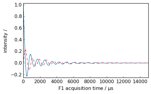
[6]:
_ = nd.plot(imag=True, xlim=(0, 5000), color="r")
_ = ndlb.plot(imag=True, data_only=True, clear=False, color="b")
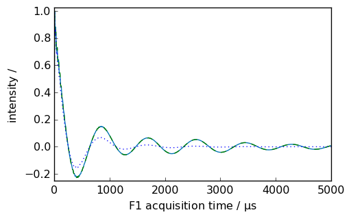
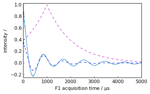
If we want to display the apodization function, we can use the retapod=True parameter.
[7]:
nd = dataset.copy()
_ = nd.plot(xlim=(0.0, 5000.0))
ndlb, apod = nd.em(
    lb=300.0 * ur.Hz, inplace=False, retapod=True
)  # ndlb contain the processed data and apod the
# apodization function
_ = ndlb.plot(data_only=True, clear=False, color="b")
_ = apod.plot(data_only=True, clear=False, color="m", linestyle="--")
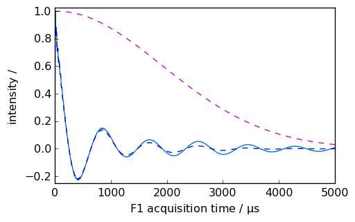
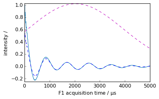
Shifted apodization
[8]:
nd = dataset.copy()
_ = nd.plot(xlim=(0.0, 5000.0))
ndlb, apod = nd.em(
    lb=300.0 * ur.Hz, shifted=1000 * ur.us, inplace=False, retapod=True
)  # ndlb contain the processed data and apod the apodization function
_ = ndlb.plot(data_only=True, clear=False, color="b")
_ = apod.plot(data_only=True, clear=False, color="m", linestyle="--")
Other apodization functions
Gaussian-Lorentzian apodization
[9]:
nd = dataset.copy()
lb = 10.0
gb = 200.0
ndlg, apod = nd.gm(lb=lb, gb=gb, inplace=False, retapod=True)
_ = nd.plot(xlim=(0.0, 5000.0))
_ = ndlg.plot(data_only=True, clear=False, color="b")
_ = apod.plot(data_only=True, clear=False, color="m", linestyle="--")
Shifted Gaussian-Lorentzian apodization
[10]:
nd = dataset.copy()
lb = 10.0
gb = 200.0
ndlg, apod = nd.gm(lb=lb, gb=gb, shifted=2000 * ur.us, inplace=False, retapod=True)
_ = nd.plot(xlim=(0.0, 5000.0))
_ = ndlg.plot(data_only=True, clear=False, color="b")
_ = apod.plot(data_only=True, clear=False, color="m", linestyle="--")
Apodization using sine window multiplication
Thesp apodization is by default performed on the last dimension.
Functional form of apodization window (cfBruker TOPSPIN manual): \(sp(t) = \sin(\frac{(\pi - \phi) t }{\text{aq}} + \phi)^{pow}\)
where * \(0 < t < \text{aq}\) and \(\phi = \pi ⁄ \text{sbb}\) when \(\text{ssb} \ge 2\)
or * \(\phi = 0\) when \(\text{ssb} < 2\)
\(\text{aq}\) is an acquisition status parameter and \(\text{ssb}\) is a processing parameter (see below) and \(\text{ pow}\) is an exponent equal to 1 for a sine bell window or 2 for a squared sine bell window.
The \(\text{ssb}\) parameter mimics the behaviour of the SSB parameter on bruker TOPSPIN software: * Typical values are 1 for a pure sine function and 2 for a pure cosine function. * Values greater than 2 give a mixed sine/cosine function. Note that all values smaller than 2, for example 0, have the same effect as \(\text{ssb}=1\), namely a pure sine function.
Shortcuts: * sine is strictly an alias of sp * sinm is equivalent to sp with \(\text{pow}=1\) * qsin is equivalent to sp with \(\text{pow}=2\)
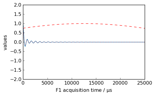
Below are several examples of sinm and qsin apodization functions.
[11]:
nd = dataset.copy()
_ = nd.plot()

new, curve = nd.qsin(ssb=3, retapod=True)
_ = curve.plot(color="r", clear=False)
_ = new.plot(xlim=(0, 25000), zlim=(-2, 2), data_only=True, color="r", clear=False)
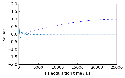
[12]:
nd = dataset.copy()
_ = nd.plot()

new, curve = nd.sinm(ssb=1, retapod=True)
_ = curve.plot(color="b", clear=False)
_ = new.plot(xlim=(0, 25000), zlim=(-2, 2), data_only=True, color="b", clear=False)
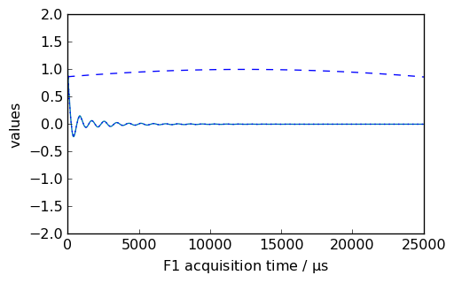
[13]:
nd = dataset.copy()
_ = nd.plot()
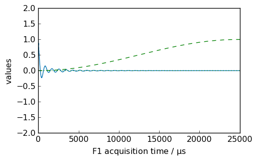
new, curve = nd.sinm(ssb=3, retapod=True)
_ = curve.plot(color="b", ls="--", clear=False)
_ = new.plot(xlim=(0, 25000), zlim=(-2, 2), data_only=True, color="b", clear=False)
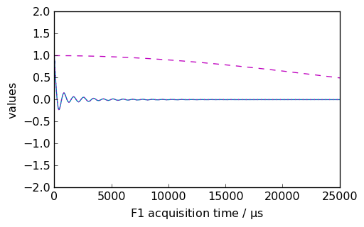
[14]:
nd = dataset.copy()
_ = nd.plot()

new, curve = nd.qsin(ssb=2, retapod=True)
_ = curve.plot(color="m", clear=False)
_ = new.plot(xlim=(0, 25000), zlim=(-2, 2), data_only=True, color="m", clear=False)
[15]:
nd = dataset.copy()
_ = nd.plot()

new, curve = nd.qsin(ssb=1, retapod=True)
_ = curve.plot(color="g", clear=False)
_ = new.plot(xlim=(0, 25000), zlim=(-2, 2), data_only=True, color="g", clear=False)