Warning

You are reading the documentation related to the development version. Go here if you are looking for the documentation of the stable release.

Principal Component Analysis

import spectrochempy as scp

SpectroChemPy's API - v.0.6.9.dev9 © Copyright 2014-2024 - A.Travert & C.Fernandez @ LCS

Introduction

PCA (standing for Principal Component Analysis) is one of the most popular method for dimensionality reduction by factorising a dataset \(X\) into score (\(S\)) and loading (\(L^T\)) matrices of a limited number of components and minimize the error \(E\):

\[X = S L^T + E\]

These matrices are such that the product of the first column of \(S\) - the score vector \(s_1\) - by the first line of \(L^T\) - the loading vector \(l_1\) - are those that best explain the variance of the dataset. These score and loading vectors are together called the ‘first component’. The second component best explain the remaining variance, etc…

The implementation of PCA in spectrochempy is based on the Scikit-Learn implementation of PCA. with similar methods and attributes on the one hands, and some that are specific to spectrochempy.

Loading of the dataset

Here we show how PCA is implemented in Scpy on a dataset corresponding to a HPLC-DAD run, from Jaumot et al. Chemolab, 76 (2005), pp. 101-110 and Jaumot et al. Chemolab, 140 (2015) pp. 1-12. This dataset (and others) can be loaded from the Multivariate Curve Resolution Homepage. For the user convenience, this dataset is present in the ‘datadir’ of spectrochempy in ‘als2004dataset.MAT’ and can be read as follows in Scpy:

A = scp.read_matlab("matlabdata/als2004dataset.MAT")

The .mat file contains 6 matrices which are thus returned in A as a list of 6 NDDatasets. We print the names and dimensions of these datasets:

for a in A:
    print(f"{a.name} : {a.shape}")

cpure : (204, 4)
MATRIX : (204, 96)
isp_matrix : (4, 4)
spure : (4, 96)
csel_matrix : (51, 4)
m1 : (51, 96)

In this tutorial, we are first interested in the dataset named (‘m1’) that contains a singleHPLC-DAD run(s). As usual, the rows correspond to the ‘time axis’ of the HPLC run(s), and the columns to the ‘wavelength’ axis of the UV spectra.

Let’s name it X (as in the matrix equation above), display its content and plot it:

X = A[-1]
X

name	m1
author	runner@fv-az1501-19
created	2024-04-28 03:09:46+02:00
history	2024-04-28 03:09:46+02:00> Imported from .mat file
DATA
title
values	[[ 0.01525 0.01285 ... 0.0003178 -0.0002631] [ 0.01969 0.01617 ... -0.007001 0.000682] ... [ 0.01 0.0144 ... -0.0007125 0.004296] [0.008121 0.01139 ... -0.007331 -0.001341]]
shape	(y:51, x:96)

_ = X.plot()

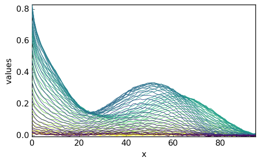
This original matrix (‘m1’) does not contain information as to the actual elution time, wavelength, and data units. Hence, the resulting NDDataset has no coordinates and on the plot, only the matrix line and row # indexes are indicated. For the clarity of the tutorial, we add: (i) a proper title to the data, (ii) the default coordinates (index) do the NDDataset and (iii) a proper name for these coordinates:

X.title = "absorbance"
X.y = scp.Coord.arange(51, title="elution time", labels=[str(i) for i in range(51)])
X.x = scp.Coord.arange(96, title="wavelength")

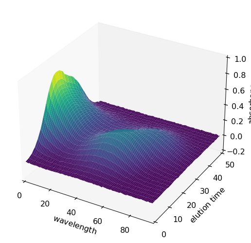
From now on, these names will be taken into account by Scpy in the plots as well as in the analysis treatments (PCA, EFA, MCR-ALS …). For instance to plot X as a surface:

surf = X.plot_surface(linewidth=0.0, ccount=100, figsize=(10, 5), autolayout=False)

Running a PCA

First, we create a PCA object with default parameters and we compute the components with the fit() method:

pca = scp.PCA()
pca.fit(X)

<spectrochempy.analysis.decomposition.pca.PCA at 0x7f7fa0d07850>

The default number of components is given by min(X.shape). As often in spectroscopy the number of observations/spectra is lower that the number of wavelength/features, the number of components often equals the number of spectra.

pca.n_components

51

As the main purpose of PCA is dimensionality reduction, we generally limit the PCA to a limited number of components. This can be done by either reseting the number of components of an existing object:

pca.n_components = 8
pca.fit(X)

<spectrochempy.analysis.decomposition.pca.PCA at 0x7f7fa0d07850>

Or directly by creating a PCA instance with the desired number of components:

pca = scp.PCA(n_components=8)
pca.fit(X)

<spectrochempy.analysis.decomposition.pca.PCA at 0x7f7fa0c32e30>

The choice of the optimum number of components to describe a dataset is always a delicate matter. It can be based on: - examination of the explained variance - examination of the scores and loadings - comparison of the experimental vs. reconstructed dataset

The so-called figures of merit of the PCA can be obtained with the printev() method: pca.printev()

The data of the two last columns are stored in the PCA.explained_variance_ratio' andPCA.cumulative_explained_variance’ attributes. They can be plotted directly as a scree plot:

_ = pca.screeplot()

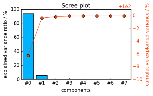
<Figure size 528x336 with 0 Axes>

The number of significant PC’s is clearly larger or equal to 2. It is, however, difficult to determine whether it should be set to 3 or 4… Let’s look at the score and loading matrices.

The scores and loadings can be obtained using the scores and loadings PCA attribute or obtained by the Scikit-Learn-like methods/attributes pca.transform() and pca.components, respectively.

Scores and Loadings can be plotted using the usual plot() method, with prior transpositon for the scores:

_ = pca.scores.T.plot()
_ = pca.loadings.plot()

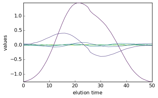
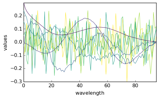
Examination of the plots above indicate that the 4th component has a structured, nonrandom loading and score, while they are random fopr the next ones. Hence, one could reasonably assume that 4 PC are enough to correctly account of the dataset.

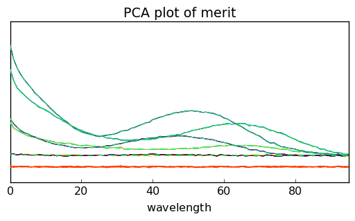
Another possibility can be a visual comparison of the modeled dataset $:nbsphinx-math:hat{X} = S L^T $, the original dataset \(X\) and the resitua,s \(E = X - \hat{X}\). This can be done using the plotmerit() method which plots both \(X\), \(\hat{X}\) (in dotted lines) and the residuals (in red):

pca = scp.PCA(n_components=4)
pca.fit(X)
_ = pca.plotmerit()

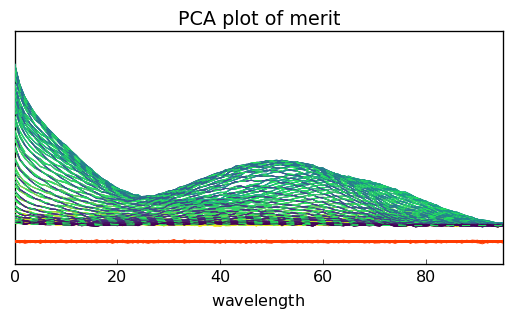
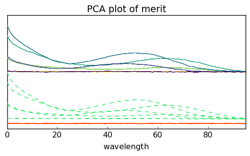
The number of spectra can be limited by the nb_traces attributes:

_ = pca.plotmerit(nb_traces=5)

and if needed both datasets can be shifted using the offset attribute (in percet of the fullscale):

pca.plotmerit(nb_traces=5, offset=100.0)

<_Axes: title={'center': 'PCA plot of merit'}, xlabel='wavelength $\\mathrm{}$', ylabel='absorbance $\\mathrm{}$'>

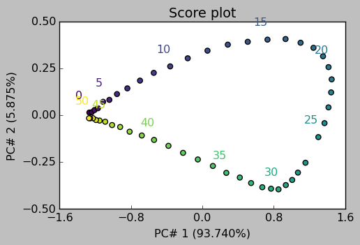
Score plots can be used to see the projection of each observation/spectrum onto the span of the principal components:

_ = pca.scoreplot(1, 2, show_labels=True, labels_every=5)
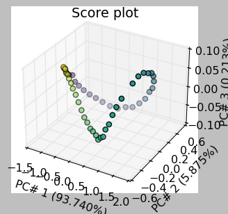
_ = pca.scoreplot(1, 2, 3)