Note
Go to the end to download the full example code.
Analysis CP NMR spectra
Example with handling of a series of CP NMR spectra.
Import API
import spectrochempy as scp
Import NMR spectra
Define the folder where are the spectra
datadir = scp.preferences.datadir
nmrdir = datadir / "nmrdata" / "bruker" / "tests" / "nmr" / "CP"
Set the glob pattern in order to load a series of spectra of given type
in the given directory (here we read fid, but we could also read “1r” files
when available)
dataset = scp.read_topspin(nmrdir, glob="**/fid")
/home/runner/work/spectrochempy/spectrochempy/src/spectrochempy/core/readers/read_topspin.py:976: UserWarning: Error reading the pulse program
  dic, data = read_fid(f_expno, acqus_files=acqus_files, procs_files=procs_files)
15 fids have been read and merged into a single dataset
The new dimension (y) have several coordinates corresponding to all metadata that change from fid to fid.
In the present case, the relevant coordinates is given by the p15 array which is the array of CP contact times.
To have y using this coordinates, we need to select it
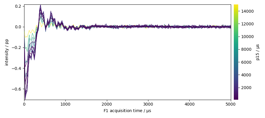
plot the dataset (zoom on the begining of the fid)
prefs = dataset.preferences
prefs.figure.figsize = (9, 4)
_ = ax = dataset.plot(colorbar=True)
_ = ax.set_xlim(0, 5000)
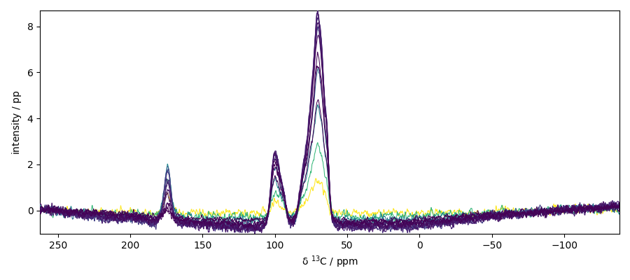
Process a fourier transform along the x dimension
fourier transform
perform a phase correction of order 0 (need to be tuned carefully)
plot
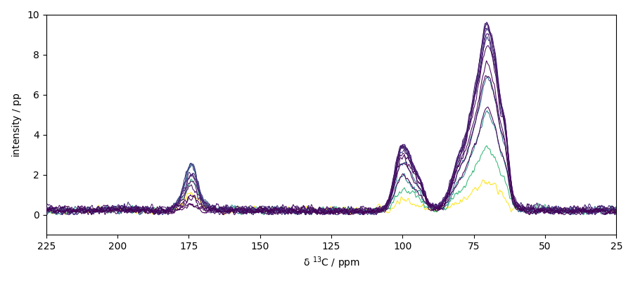
## Baseline correction Here we use the snip algorithm
nd4 = scp.snip(nd3, snip_width=200)

ax = nd4.plot()
_ = ax.set_xlim(225, 25)
_ = ax.set_ylim(-1, 10)
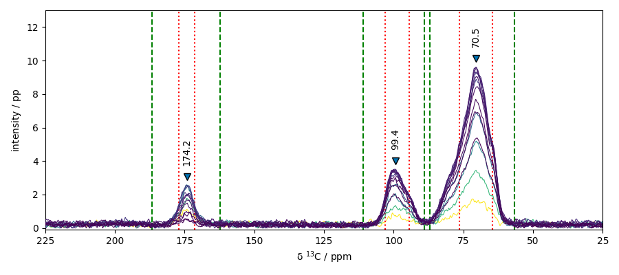
## Peak peaking we will use here the max of each spectra
peaks, properties = nd4.max(dim=0).find_peaks(height=2.0, width=0.5, wlen=33.0)
print(f"position of the peaks : {peaks.x.data}")
position of the peaks : [ 174.2 99.38 70.46]
properties of the peaks
table_pos = "  ".join([f"{peaks[i].x.value.m:>10.3f}" for i in range(len(peaks))])
print(f"{'peak_position (cm⁻¹)':>26}: {table_pos}")
for key in properties:
    table_property = "  ".join(
        [f"{properties[key][i].m:>10.3f}" for i in range(len(peaks))]
    )
    title = f"{key:>.16} ({properties[key][0].u:~P})"
    print(f"{title:>26}: {table_property}")
peak_position (cm⁻¹):    174.243      99.379      70.458
   peak_heights (pp):      2.579       3.516       9.606
    prominences (pp):      2.242       3.069       9.028
    left_bases (ppm):    186.765     110.857      86.891
   right_bases (ppm):    162.408      88.945      56.763
        widths (ppm):      5.575       8.569      11.783
  width_heights (pp):      1.458       1.982       5.092
      left_ips (ppm):    177.015     103.010      76.346
     right_ips (ppm):    171.440      94.441      64.562
plot with peak markers and the left/right-bases indicators
ax = nd4.plot()  # output the spectrum on ax. ax will receive next plot too
pks = peaks + 0.5  # add a small offset on the y position of the markers
_ = pks.plot_scatter(
    ax=ax,
    marker="v",
    color="black",
    clear=False,  # we need to keep the previous output on ax
    data_only=True,  # we don't need to redraw all things like labels, etc...
    ylim=(-0.1, 13),
    xlim=(225, 25),
)

for i, p in enumerate(pks):
    x, y = p.x.values, (p + 0.5).values
    _ = ax.annotate(
        f"{x.m:0.1f}",
        xy=(x, y),
        xytext=(-5, 5),
        rotation=90,
        textcoords="offset points",
    )
    for w in (properties["left_bases"][i], properties["right_bases"][i]):
        ax.axvline(w, linestyle="--", color="green")
    for w in (properties["left_ips"][i], properties["right_ips"][i]):
        ax.axvline(w, linestyle=":", color="red")
Get the section at once using fancy indexing
sections = nd4[:, peaks.x.data]

# The array sections has a shape (15, 3).
# We must transpose it to plot the three sections has a function of contact time
sections = sections.T

# now plot it
ax = sections.plot(marker="o", lw="1", ls=":", legend="best", colormap="jet")
_ = ax.set_xlim(0, 16000)
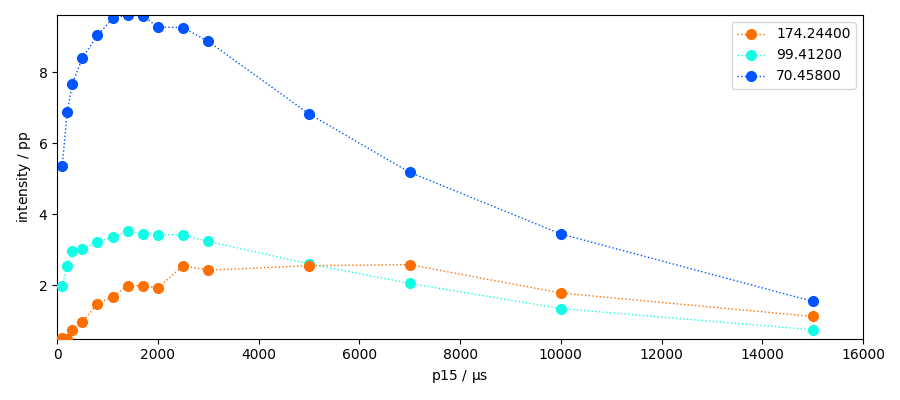
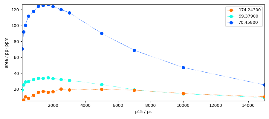
The sections we have taken here represent the maximum heigths of the peaks. However it could may be interesting to have the area of the peak instead. Let’s use the left and right bases to perform the integration of the peaks.
area = []
for i in range(len(peaks)):
    lb, ub = properties["left_bases"][i].m, properties["right_bases"][i].m
    a = nd4[:, lb:ub].simpson()
    area.append(a)

area = scp.NDDataset(
    area,
    dims=["y", "x"],
    coordset=scp.CoordSet({"y": peaks.x.copy(), "x": nd4.y.default.copy()}),
    units=a.units,
    title="area",
)
area.plot(marker="o", lw="1", ls=":", legend="best", colormap="jet")
area
Fitting a model to these data
import numpy as np

# create an Optimize object using a simple leastsq method
fitter = scp.Optimize(log_level="INFO", method="leastsq")


# define a model
# Note: This is only for sake of demonstration,
# as the model is probably not sufficient to fit the data correctly.
def cp_model(t, i0, tis, t1irho):  # warning: no underscore in variable names
    I = i0 * (np.exp(-t / t1irho) - np.exp(-t * (1 / tis))) / (1 - tis / t1irho)
    return I


# Add the model to the fitter usermodels as it it not a built-in model
fitter.usermodels = {"CP_model": cp_model}
index = 0
s = area[index]

# Define the parameter variables using a script
# (parameter: value, low_bound,  high_bound)
# - no underscore in parameters names.
# - times are in the units of the data time coordinates (here `s`)
# - initially we assume relaxation (T1rho) time constant vey large
fitter.script = """
 MODEL: cp
 shape: cp_model
    $ i0:     25, 0.1, none
    $ t1irho: 1e4, 1, none
    $ tis:  800, 1, 10000
"""

_ = fitter.fit(s)

spred = fitter.predict()

ax = fitter.plotmerit(
    s,
    spred,
    method="scatter",
    show_yaxis=True,
    title=f"fitting CP dynamic (peaks at {peaks.x[index].values})",
)
_ = ax.set_xlim(0, 16000)
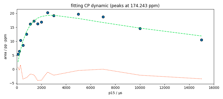
**************************************************
Result:
**************************************************


MODEL: cp
shape: cp_model
       $ i0:    19.2907, 0.1, none
       $ t1irho: 23482.1106, 1, none
       $ tis:   796.2717, 1, 10000
index = 1
s = area[index]
fitter.script = """
 MODEL: cp
 shape: cp_model
    $ i0:     35, 0.1, none
    $ t1irho: 1e4, 1, none
    $ tis:  800, 1, 10000
"""

_ = fitter.fit(s)

spred = fitter.predict()

ax = fitter.plotmerit(
    s,
    spred,
    method="scatter",
    show_yaxis=True,
    title=f"fitting CP dynamic (peaks at {peaks.x[index].values})",
)
_ = ax.set_xlim(0, 16000)
**************************************************
Result:
**************************************************


MODEL: cp
shape: cp_model
       $ i0:    34.7742, 0.1, none
       $ t1irho: 11463.4262, 1, none
       $ tis:   174.4446, 1, 10000
index = 2
s = area[index]
fitter.script = """
 MODEL: cp
 shape: cp_model
    $ i0:     125, 0.1, none
    $ t1irho: 1e4, 1, none
    $ tis:  800, 1, 10000
"""

_ = fitter.fit(s)

spred = fitter.predict()

ax = fitter.plotmerit(
    s,
    spred,
    method="scatter",
    show_yaxis=True,
    title=f"fitting CP dynamic (peaks at {peaks.x[index].values})",
)
_ = ax.set_xlim(0, 16000)
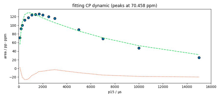
**************************************************
Result:
**************************************************


MODEL: cp
shape: cp_model
       $ i0:   129.5282, 0.1, none
       $ t1irho: 10031.3641, 1, none
       $ tis:   196.1622, 1, 10000
The model looks good for the peak at 174 ppm. This peak appears to be composed of a single species, which is not the case for the other peaks at 99 and 70 ppm. Deconvolution of these two peaks is therefore probably necessary for a better analysis.
This ends the example ! The following line can be removed or commented
when the example is run as a notebook (ipynb).
# scp.show()
Total running time of the script: (0 minutes 3.304 seconds)