FTIR interferogram processing

A situation where we need transform of real data is the case of FTIR interferogram.

import spectrochempy as scp
from spectrochempy.core.units import ur

SpectroChemPy's API - v.0.7.1 © Copyright 2014-2025 - A.Travert & C.Fernandez @ LCS

ir = scp.read_spa("irdata/interferogram/interfero.SPA")

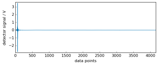
By default, the interferogram is displayed with an axis in points (no units).

prefs = ir.preferences
prefs.figure.figsize = (7, 3)
_ = ir.plot()
print("number of points = ", ir.size)

number of points =  4160

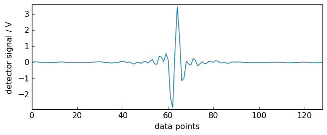
Plotting a zoomed region around the maximum of the interferogram (the so-called ZPD: Zero optical Path Difference ) we can see that it is located around the 64th points. The FFT processing will need this information, but it will be determined automatically.

_ = ir.plot(xlim=(0, 128))

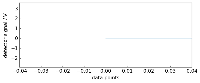
The x scale of the interferogram can also be displayed as a function of optical path difference. For this we just make show_datapoints to False:

ir.x.show_datapoints = False
_ = ir.plot(xlim=(-0.04, 0.04))

Note that the x scale of the interferogram has been calculated using the laser frequency indicated in the original omnic file. It is stored in the meta attribute of the NDDataset:

print(ir.meta.laser_frequency)

15798.259765625 cm⁻¹

If absent, it can be set using the set_laser_frequency() method, e.g.:

ir.x.set_laser_frequency(15798.26 * ur("cm^-1"))

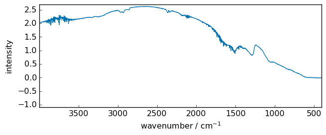
Now we can perform the Fourier transform. By default, no zero-filling level is applied prior the Fourier transform for FTIR. To add some level of zero-filling, use the zf method.

ird = ir.dc()
ird = ird.zf(size=2 * ird.size)
irt = ird.fft()

_ = irt.plot(xlim=(3999, 400))

 WARNING | (DeprecationWarning) Conversion of an array with ndim > 0 to a scalar is deprecated, and will error in future. Ensure you extract a single element from your array before performing this operation. (Deprecated NumPy 1.25.)
 WARNING | (RuntimeWarning) divide by zero encountered in divide

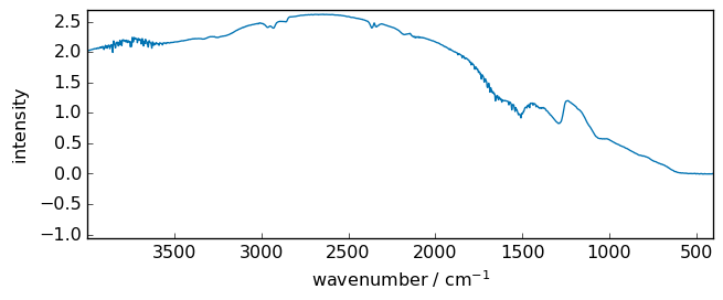
A Happ-Genzel (Hamming window) apodization can also be applied prior to the Fourier transformation in order to decrease the H2O narrow bands.

ird = ir.dc()
irdh = ird.hamming()
irdh.zf(inplace=True, size=2 * ird.size)
irth = irdh.fft()
_ = irth.plot(xlim=(3999, 400))

 WARNING | (DeprecationWarning) Conversion of an array with ndim > 0 to a scalar is deprecated, and will error in future. Ensure you extract a single element from your array before performing this operation. (Deprecated NumPy 1.25.)
 WARNING | (DeprecationWarning) Conversion of an array with ndim > 0 to a scalar is deprecated, and will error in future. Ensure you extract a single element from your array before performing this operation. (Deprecated NumPy 1.25.)
 WARNING | (RuntimeWarning) divide by zero encountered in divide

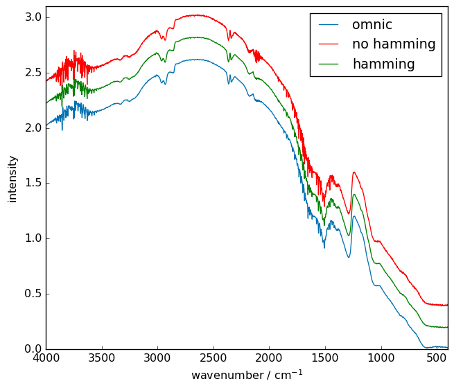
Comparison with the OMNIC processing.

Here we compare the OMNIC processed spectra of the same interferogram and ours in red. One can see that the results are very close

irs = scp.read_spa("irdata/interferogram/spectre.SPA")
prefs.figure.figsize = (7, 6)
ax = irs.plot(label="omnic")
(irt + 0.4).plot(c="red", linestyle="solid", clear=False, label="no hamming")
(irth + 0.2).plot(c="green", linestyle="solid", clear=False, label="hamming")
ax.set_xlim(4000.0, 400.0)
ax.set_ylim(0.0, 3.1)
_ = ax.legend()