spectrochempy.EFA

class EFA(*, log_level='WARNING', warm_start=False, cutoff=None, n_components=None)[source][source]

Evolving Factor Analysis (EFA).

Evolving factor analysis (EFA) is a method that allows model-free resolution of overlapping peaks into concentration profiles and normalized spectra of components.

Originally developed for GC and GC-MS experiments (See e.g., Maeder and Zuberbuehler [1986] , Roach and Guilhaus [1992]), it is also suitable for analysis spectra such as those obtained by Operando FTIR for example.

The model used in this class allow to perform a forward and reverse analysis of the input NDDataset .

Parameters:

log_level (any of ["INFO", "DEBUG", "WARNING", "ERROR"], optional, default: "WARNING") – The log level at startup. It can be changed later on using the set_log_level method or by changing the log_level attribute.
warm_start (bool, optional, default: False) – When fitting repeatedly on the same dataset, but for multiple parameter values (such as to find the value maximizing performance), it may be possible to reuse previous model learned from the previous parameter value, saving time.

When warm_start is True, the existing fitted model attributes is used to initialize the new model in a subsequent call to fit.
cutoff (float, optional, default: None) – Cut-off value.
n_components (int, optional, default: None) – Number of components to keep.

See also

FastICA: Perform Independent Component Analysis with a fast algorithm.
IRIS: Integral inversion solver for spectroscopic data.
MCRALS: Perform MCR-ALS of a dataset knowing the initial \(C\) or \(S^T\) matrix.
NMF: Non-Negative Matrix Factorization.
PCA: Perform Principal Components Analysis.
SIMPLISMA: SIMPLe to use Interactive Self-modeling Mixture Analysis.
SVD: Perform a Singular Value Decomposition.

Examples

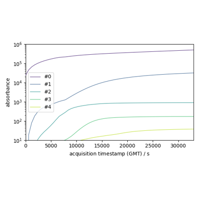
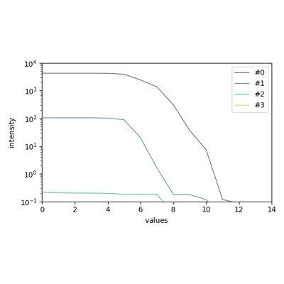
>>> # Init the model
>>> model = scp.EFA()
>>> # Read an experimental 2D spectra (N x M )
>>> X = scp.read("irdata/nh4y-activation.spg")
>>> # Fit the model
>>> _ = model.fit(X)
>>> # Display components spectra (2 x M)
>>> model.n_components = 2
>>> _ = model.components.plot(title="Component spectra")
>>> # Get the abstract concentration profile based on the FIFO EFA analysis
>>> c = model.transform()
>>> # Plot the transposed concentration matrix  (2 x N)
>>> _ = c.T.plot(title="Concentration")
>>> scp.show()

Initialize the BaseConfigurable class.

Parameters:

log_level (int, optional) – The log level at startup. Default is logging.WARNING.
**kwargs (dict) – Additional keyword arguments for configuration.

Attributes Summary

`X`	Return the X input dataset (eventually modified by the model).
`Y`	The `Y` input.
`b_ev`	Eigenvalues for the backward analysis ( `NDDataset` ).
`components`	`NDDataset` with components in feature space (n_components, n_features).
`config`	`traitlets.config.Config` object.
`cutoff`	Cut-off value.
`f_ev`	Eigenvalues for the forward analysis ( `NDDataset` ).
`log`	Return `log` output.
`n_components`	Number of components to keep.
`name`	Object name

Methods Summary

`fit`(X)	Fit the `EFA` model on a `X` dataset.
`fit_transform`(X, **kwargs)	Fit the model with X and apply the dimensionality reduction on X.
`get_components`([n_components])	Return the component's dataset: (selected n_components, n_features).
`inverse_transform`()	Not implemented.
`parameters`([replace, removed, default])	Alias for `params` method.
`params`([default])	Return current or default configuration values.
`plotmerit`([X, X_hat])	Plot the input (`X`), reconstructed (`X_hat`) and residuals.
`reconstruct`()	Not implemented.
`reduce`([X])	Apply dimensionality reduction to `X`.
`reset`()	Reset configuration parameters to their default values.
`to_dict`()	Return config value in a dict form.
`transform`([X])	Apply dimensionality reduction to `X`.

Attributes Documentation

X: Return the X input dataset (eventually modified by the model).

Y: The Y input.

b_ev: Eigenvalues for the backward analysis ( NDDataset ).

components

NDDataset with components in feature space (n_components, n_features).

See also

fit_transform: Fit the model with an input dataset X and apply the dimensionality reduction on X.
fit_reduce: Alias of fit_transform (Deprecated).

fit_transform(X, **kwargs)[source][source]

Fit the model with X and apply the dimensionality reduction on X.

Parameters:

X (NDDataset or array-like of shape (n_observations, n_features)) – Training data.
**kwargs (keyword parameters, optional) – See Other Parameters.

Returns:

NDDataset – Dataset with shape (n_observations, n_components).

Other Parameters:

n_components (int, optional) – The number of components to use for the reduction. If not given the number of components is eventually the one specified or determined in the fit process.

get_components(n_components=None)

Return the component’s dataset: (selected n_components, n_features).

Parameters:: n_components (int, optional, default: None) – The number of components to keep in the output dataset. If None, all calculated components are returned.
Returns:: NDDataset – Dataset with shape (n_components, n_features)

inverse_transform()[source][source]: Not implemented.

parameters(replace="params", removed="0.7.1") def parameters(self, default=False)[source]: Alias for params method.

params(default=False)[source]

Return current or default configuration values.

Parameters:: default (bool, optional, default: False) – If default is True, the default parameters are returned, else the current values.
Returns:: dict – Current or default configuration values.

plotmerit(X=None, X_hat=None, **kwargs)[source]

Plot the input (X), reconstructed (X_hat) and residuals.

\(X\) and \(\hat{X}\) can be passed as arguments. If not, the X attribute is used for \(X`and :math:\)hat{X}`is computed by the inverse_transform method

Parameters:

X (NDDataset, optional) – Original dataset. If is not provided (default), the X attribute is used and X_hat is computed using inverse_transform.
X_hat (NDDataset, optional) – Inverse transformed dataset. if X is provided, X_hat must also be provided as compuyed externally.
**kwargs (keyword parameters, optional) – See Other Parameters.

Returns:

Axes – Matplotlib subplot axe.

Other Parameters:

colors (tuple or ndarray of 3 colors, optional) – Colors for X , X_hat and residuals E . in the case of 2D, The default colormap is used for X . By default, the three colors are NBlue , NGreen and NRed (which are colorblind friendly).
offset (float, optional, default: None) – Specify the separation (in percent) between the \(X\) , \(X_hat\) and \(E\).
nb_traces (int or 'all', optional) – Number of lines to display. Default is 'all'.
**others (Other keywords parameters) – Parameters passed to the internal plot method of the X dataset.

reconstruct()[source][source]: Not implemented.

reduce(X=None, **kwargs)[source]

Apply dimensionality reduction to X.

Parameters:

X (NDDataset or array-like of shape (n_observations, n_features), optional) – New data, where n_observations is the number of observations and n_features is the number of features. if not provided, the input dataset of the fit method will be used.
**kwargs (keyword parameters, optional) – See Other Parameters.

Returns:

NDDataset – Dataset with shape (n_observations, n_components).

Other Parameters:

n_components (int, optional) – The number of components to use for the reduction. If not given the number of components is eventually the one specified or determined in the fit process.

Notes

Deprecated in version 0.6.

reset()[source]: Reset configuration parameters to their default values.

to_dict()[source]

Return config value in a dict form.

Returns:: dict – A regular dictionary.

transform(X=None, **kwargs)

Apply dimensionality reduction to X.

Parameters:

X (NDDataset or array-like of shape (n_observations, n_features), optional) – New data, where n_observations is the number of observations and n_features is the number of features. if not provided, the input dataset of the fit method will be used.
**kwargs (keyword parameters, optional) – See Other Parameters.

Returns:

NDDataset – Dataset with shape (n_observations, n_components).

Other Parameters:

n_components (int, optional) – The number of components to use for the reduction. If not given the number of components is eventually the one specified or determined in the fit process.

Examples using spectrochempy.EFA

EFA example

EFA (Keller and Massart original example)

MCR-ALS with kinetic constraints