Processing NMR spectra (slicing, baseline correction, peak picking, peak fitting)

Various examples of processing NMR spectra

Import API

import spectrochempy as scp

Importing a 2D NMR spectra

Define the folder where are the spectra

datadir = scp.preferences.datadir
nmrdir = datadir / "nmrdata"

dataset = scp.read_topspin(
    nmrdir / "bruker" / "tests" / "nmr" / "topspin_2d" / "1" / "pdata" / "1" / "2rr"
)

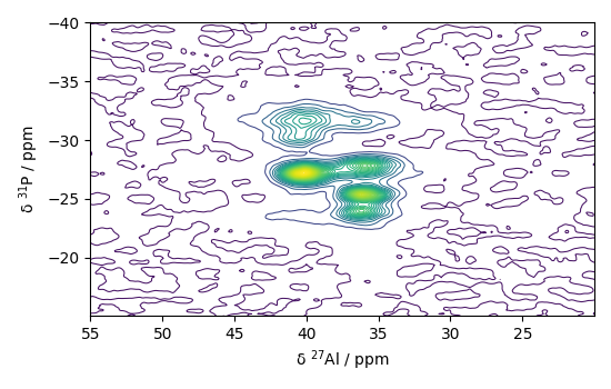
Analysing the 2D NMD dataset

Print dataset summary

dataset

name	topspin_2d expno:1 procno:1 (2D)
author	runner@fv-az1774-299
created	2025-02-25 07:59:05+00:00
DATA
title	intensity
values	RR[[ 0.1001 0.1188 ... 0.009276 -0.03083] [ 0.08574 0.1094 ... 0.02799 -0.01425] ... [ 0.1134 0.1161 ... -0.03438 -0.06006] [ 0.1091 0.1206 ... -0.01183 -0.04616]] pp RI[[ -0.1092 -0.07951 ... 0.1269 0.1117] [ -0.1287 -0.1068 ... 0.1194 0.1155] ... [-0.06948 -0.03049 ... 0.1292 0.09699] [-0.08905 -0.05339 ... 0.1305 0.1055]] pp IR[[ 0.0913 0.06793 ... -0.1012 -0.118] [ 0.08804 0.06219 ... -0.09448 -0.1108] ... [ 0.09555 0.08065 ... -0.1116 -0.1259] [ 0.09386 0.07434 ... -0.1068 -0.1229]] pp II[[-0.06389 -0.07123 ... 0.09588 0.09539] [-0.07548 -0.07779 ... 0.1075 0.1114] ... [-0.04044 -0.05341 ... 0.0732 0.06366] [-0.05242 -0.06344 ... 0.08463 0.07955]] pp
shape	(y:1024(complex), x:2048(complex))
DIMENSION `x`
size	2048
title	$\delta\ ^{27}Al$
coordinates	[ 96.79 96.7 ... -102.8 -102.9] ppm
DIMENSION `y`
size	1024
title	$\delta\ ^{31}P$
coordinates	[ 38.79 38.7 ... -44.52 -44.6] ppm

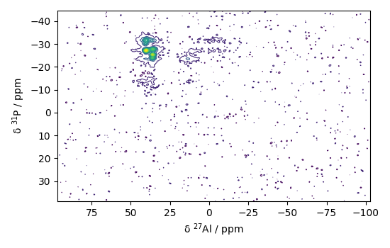
Plot the dataset

_ = dataset.plot_map()

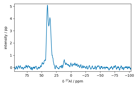
Extract slices along x

s = dataset[-27.6, :]
_ = s.plot()

Baseline correction of this slice Note that only the real part is corrected

sa = s.snip(snip_width=100)
_ = sa.plot()

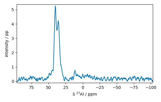
apply this correction to the whole dataset

sb = dataset.snip(snip_width=100)
_ = sb.plot_map()

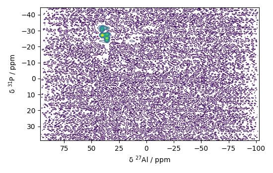
Select a region of interest

sc = sb[
    -40.0:-15.0, 55.0:20.0
]  # note the use of float to make selection using coordinates (not point indexes)
_ = sc.plot_map()

Extract slices along x

s1 = sc[-27.6, :]
_ = s1.plot()

s2 = sc[-25.7, :]
_ = s2.plot()

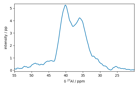
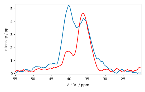
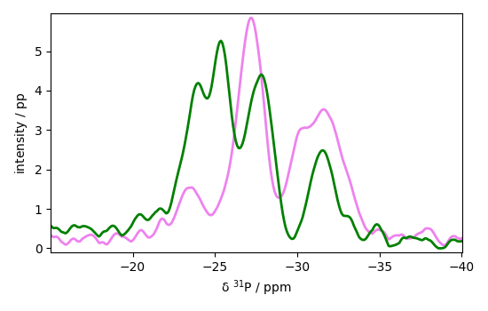
plot two slices on the same figure

_ = s1.plot()
_ = s2.plot(
    clear=False,
    color="red",
    linestyle="-",
)

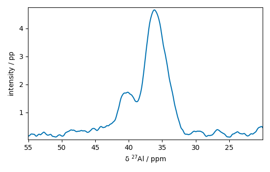
Now slice along y

s3 = sc[:, 40.0]
s4 = sc[:, 36.0]

IMPORTANT: note that when the slice is along y, this results in a column vector of shape (308, 1). When an NDDataset method is applied to this slice, such as a baseline correction, it will be applied by default to the last dimension [rows] (in this case the dimension of size 1, which is not what is generally expected). To avoid this, we can use the squeeze method to remove this dimension or transpose the slice to obtain a vector of rows of shape (1, 308)

s3 = s3.squeeze()
s4 = s4.squeeze()

plot the two slices on the same figure

_ = s3.plot(color="violet", ls="-", lw="2")
_ = s4.plot(clear=False, color="green", ls="-", lw="2")

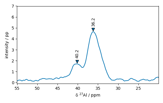
Peak picking

peaks, _ = s2.find_peaks()

plot the position of the peaks For this we will define a plot function that we be reused later

def plot_with_pp(s, peaks):
    ax = s.plot()  # output the spectrum on ax. ax will receive next plot too
    pks = peaks + 0.2  # add a small offset on the y position of the markers
    _ = pks.plot_scatter(
        ax=ax,
        marker="v",
        color="black",
        clear=False,  # we need to keep the previous output on ax
        data_only=True,  # we don't need to redraw all things like labels, etc...
        ylim=(-0.1, 7),
    )

    for p in pks:
        x, y = p.coord(-1).values, (p + 0.2).values
        _ = ax.annotate(
            f"{x.m:0.1f}",
            xy=(x, y),
            xytext=(-5, 5),
            rotation=90,
            textcoords="offset points",
        )


_ = plot_with_pp(s2, peaks)

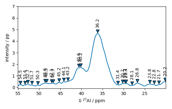
Set some parameters to get less but significant peaks

peaks, _ = s2.find_peaks(height=1.0, distance=1.0)
_ = plot_with_pp(s2, peaks)

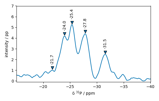
Now look in the other dimension using slice s4

peaks, _ = s4.find_peaks(height=1.0, distance=1.0)
_ = plot_with_pp(s4, peaks)

Peak fitting

Fit parameters are defined in a script (a single text as below)

script = """
#-----------------------------------------------------------
# syntax for parameters definition:
# name: value, low_bound,  high_bound
# available prefix:
#  # for comments
#  * for fixed parameters
#  $ for variable parameters
#  > for reference to a parameter in the COMMON block
#    (> is forbidden in the COMMON block)
# common block parameters should not have a _ in their names
#-----------------------------------------------------------
#

COMMON:
$ commonwidth: 1, 0, 5
$ commonratio: .5, 0, 1

MODEL: LINE_1
shape: voigtmodel
    $ ampl:  1, 0.0, none
    $ pos:   -21.7, -22., -20
    > ratio: commonratio
    > width: commonwidth

MODEL: LINE_2
shape: voigtmodel
    $ ampl:  4, 0.0, none
    $ pos:   -24, -24.5, -23.5
    > ratio: commonratio
    > width: commonwidth

MODEL: LINE_3
shape: voigtmodel
    $ ampl:  4, 0.0, none
    $ pos:   -25.4, -25.8, -25
    > ratio: commonratio
    > width: commonwidth

MODEL: LINE_4
shape: voigtmodel
    $ ampl:  4, 0.0, none
    $ pos:   -27.8, -28.5, -27
    > ratio: commonratio
    > width: commonwidth

MODEL: LINE_5
shape: voigtmodel
    $ ampl:  4, 0.0, none
    $ pos:   -31.5, -32, -31
    > ratio: commonratio
    > width: commonwidth

"""

We will work here on the slice s4 (taken in the y dimension).

s4p = s4.snip()  # Baseline correction

create an Optimize object

f1 = scp.Optimize(log_level="INFO")

Set parameters

f1.script = script
f1.max_iter = 5000

Fit the slice s4p

_ = f1.fit(s4p)

**************************************************
Result:
**************************************************

COMMON:
       $ commonwidth:     1.8757, 0, 5
       $ commonratio:     0.7139, 0, 1

MODEL: line_1
shape: voigtmodel
       $ ampl:     0.4913, 0.0, none
       $ pos:   -21.0847, -22.0, -20
       > ratio:commonratio
       > width:commonwidth

MODEL: line_2
shape: voigtmodel
       $ ampl:     3.1380, 0.0, none
       $ pos:   -23.7153, -24.5, -23.5
       > ratio:commonratio
       > width:commonwidth

MODEL: line_3
shape: voigtmodel
       $ ampl:     4.2827, 0.0, none
       $ pos:   -25.3868, -25.8, -25
       > ratio:commonratio
       > width:commonwidth

MODEL: line_4
shape: voigtmodel
       $ ampl:     4.1165, 0.0, none
       $ pos:   -27.7584, -28.5, -27
       > ratio:commonratio
       > width:commonwidth

MODEL: line_5
shape: voigtmodel
       $ ampl:     2.3106, 0.0, none
       $ pos:   -31.5949, -32, -31
       > ratio:commonratio
       > width:commonwidth

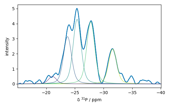
Show the result

s4p.plot()
ax = (f1.components[:]).plot(clear=False)
ax.autoscale(enable=True, axis="y")

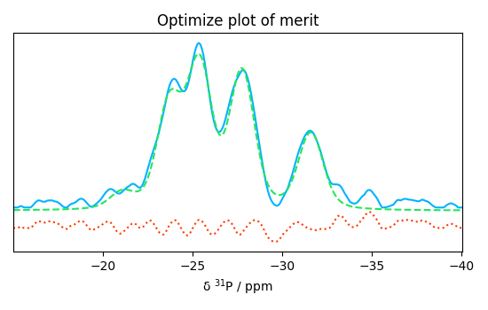
# Plotmerit
som = f1.inverse_transform()
_ = f1.plotmerit(offset=2)

• 
• 

This ends the example ! The following line can be removed or commented when the example is run as a notebook (ipynb).

# scp.show()