EFA example

In this example, we perform the Evolving Factor Analysis

sphinx_gallery_thumbnail_number = 2

import os

import spectrochempy as scp

Upload and preprocess a dataset

datadir = scp.preferences.datadir
dataset = scp.read_omnic(os.path.join(datadir, "irdata", "nh4y-activation.spg"))

Change the time origin

dataset.y -= dataset.y[0]

columns masking

dataset[:, 1230.0:920.0] = scp.MASKED  # do not forget to use float in slicing
dataset[:, 5997.0:5993.0] = scp.MASKED

difference spectra dataset -= dataset[-1]

dataset.plot_stack(title="NH4_Y activation dataset")

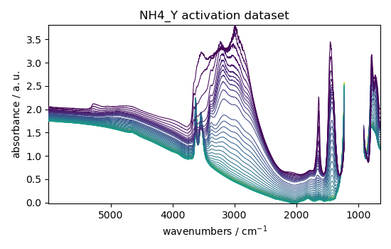
<_Axes: title={'center': 'NH4_Y activation dataset'}, xlabel='wavenumbers $\\mathrm{/\\ \\mathrm{cm}^{-1}}$', ylabel='absorbance $\\mathrm{/\\ \\mathrm{a.u.}}$'>

Evolving Factor Analysis

efa1 = scp.EFA()
_ = efa1.fit(dataset)

Forward evolution of the 5 first components

f = efa1.f_ev[:, :5]
f.T.plot(yscale="log", legend=f.x.labels)

# Backward evolution
b = efa1.b_ev[:, :5]
b.T[:5].plot(yscale="log", legend=b.x.labels)

• 
• 

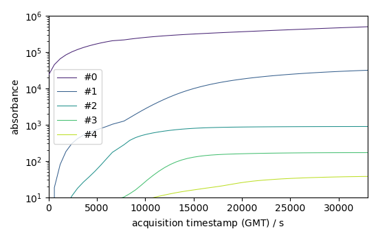
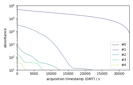
<_Axes: xlabel='acquisition timestamp (GMT) $\\mathrm{/\\ \\mathrm{s}}$', ylabel='absorbance $\\mathrm{}$'>

Show results with 3 components (which seems to already explain a large part of the dataset) we use the magnitude of the 4th component for the cut-off value (assuming it corresponds mostly to noise)

efa1.n_components = 3
efa1.cutoff = efa1.f_ev[:, 3].max()

# get concentration
C1 = efa1.transform()
C1.T.plot(title="EFA determined concentrations", legend=C1.x.labels)

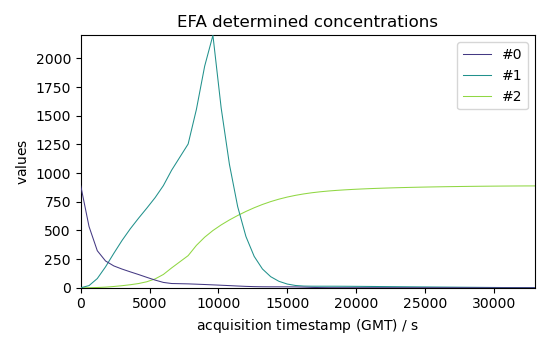
<_Axes: title={'center': 'EFA determined concentrations'}, xlabel='acquisition timestamp (GMT) $\\mathrm{/\\ \\mathrm{s}}$', ylabel='values $\\mathrm{}$'>

Fit transform : Get the concentration in too commands The number of desired components can be passed to the EFA model, followed by the fit_transform method:

efa2 = scp.EFA(n_components=3)
C2 = efa2.fit_transform(dataset)
assert C1 == C2

Get components

St = efa2.get_components()
St.plot(title="components", legend=St.y.labels)

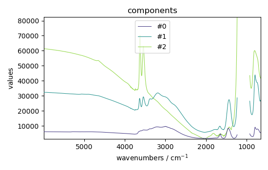
<_Axes: title={'center': 'components'}, xlabel='wavenumbers $\\mathrm{/\\ \\mathrm{cm}^{-1}}$', ylabel='values $\\mathrm{}$'>

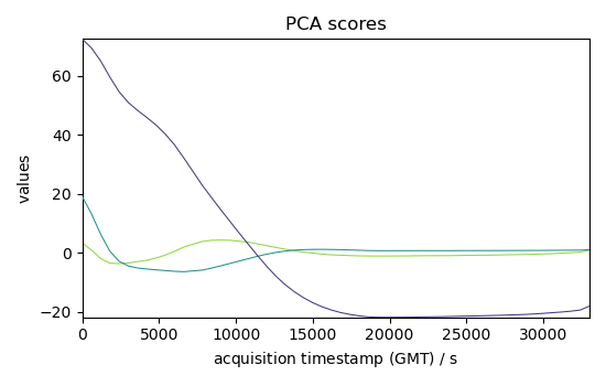
Compare with PCA

pca = scp.PCA(n_components=3)
C3 = pca.fit_transform(dataset)

C3.T.plot(title="PCA scores")

<_Axes: title={'center': 'PCA scores'}, xlabel='acquisition timestamp (GMT) $\\mathrm{/\\ \\mathrm{s}}$', ylabel='values $\\mathrm{}$'>

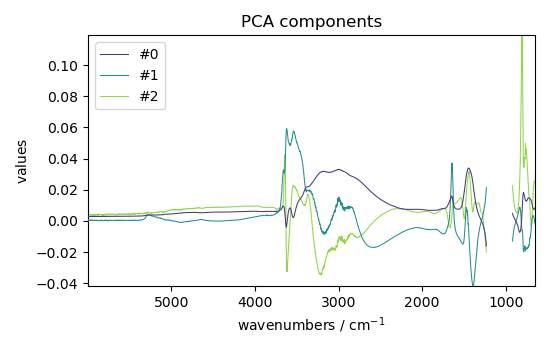
LT = pca.loadings
LT.plot(title="PCA components", legend=LT.y.labels)

<_Axes: title={'center': 'PCA components'}, xlabel='wavenumbers $\\mathrm{/\\ \\mathrm{cm}^{-1}}$', ylabel='values $\\mathrm{}$'>

This ends the example ! The following line can be uncommented if no plot shows when running the .py script

# scp.show()