Solve a linear equation using LSTSQ

In this example, we find the least square solution of a simple linear equation.

# sphinx_gallery_thumbnail_number = 2

import spectrochempy as scp

Let’s take a similar example to the one given in the numpy.linalg documentation

We have some noisy data that represent the distance d traveled by some objects versus time t:

time = [0, 1, 2, 3]
distance = [-1, 0.2, 0.9, 2.1]

### 1) Using arrays (or list) inputs

We would like v and d0 such as

distance = v.time + d0

lstsq = scp.LSTSQ()
lstsq.fit(time, distance)
v = lstsq.coef
d0 = lstsq.intercept
rsquare = lstsq.score()
v, d0, rsquare

(0.9999999999999997, -0.9499999999999995, 0.9900990099009901)

Plot (we need to import the matplotlib library)

import matplotlib.pyplot as plt

plt.plot(time, distance, "o", label="Original data", markersize=5)
distance_fitted = lstsq.predict()
plt.plot(time, distance_fitted, ":r", label="Linear regression output")
plt.xlabel("time / h")
plt.ylabel("distance / km")
plt.title(f"Linear regression, $R^2={rsquare:.3f}$")
plt.legend()

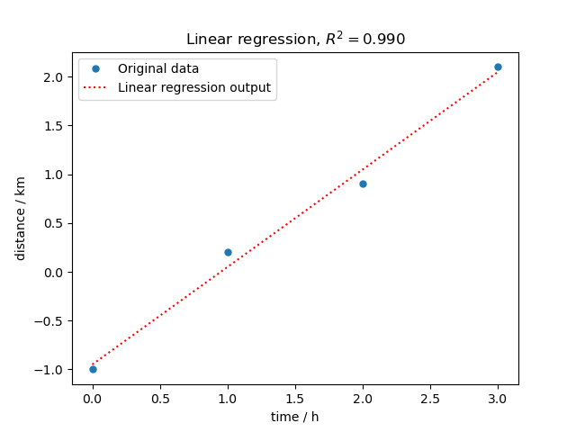
<matplotlib.legend.Legend object at 0x7f15af879310>

### 2) Using NDDataset as input for X and Y

Using NDDataset as input offer the straightforward possibility to use metadata such as units in the calculation and coordset

time = scp.NDDataset([0, 1, 2, 3], title="time", units="hour")
distance = scp.NDDataset([-1, 0.2, 0.9, 2.1], title="distance", units="kilometer")

we fit it using the new defined time and distance NDDatasets

lstsq = scp.LSTSQ()
lstsq.fit(time, distance)

# The results are the same as previously (but with units information)
v = lstsq.coef
d0 = lstsq.intercept
rsquare = lstsq.score()
print(f"speed : {v:.2fK},  d0 : {d0:.2fK},  r^2={rsquare:.3f}")

speed : 1.00 kilometer.hour^-1,  d0 : -0.95 kilometer,  r^2=0.990

Predict return a NDDataset since the inputs were NDDatasets

distance_fitted2 = lstsq.predict()
print(distance_fitted2)

assert (distance_fitted == distance_fitted2.data).all()

NDDataset: [float64] km (size: 4)

### 3) Using a single NDDataset with X coordinates as input

Using NDDataset as input offer the straightforward possibility to use the X coordinate directly, ie., we use lstsq.fit(Y) with Y.x = X, instead of lstsq.fit(X, Y)

time = scp.Coord([0, 1, 2, 3], title="time", units="hour")
distance = scp.NDDataset(
    data=[-1, 0.2, 0.9, 2.1], coordset=[time], title="distance", units="kilometer"
)

Now we fit the model, but here we just need to pass the distance dataset as argument. The time information being the x coordinates.

lstsq = scp.LSTSQ()
lstsq.fit(distance)

# The results are the same as previously.
v = lstsq.coef
d0 = lstsq.intercept
rsquare = lstsq.score()
print(f"speed : {v:.2fK},  d0 : {d0:.2fK},  r^2={rsquare:.3f}")

speed : 1.00 kilometer.hour^-1,  d0 : -0.95 kilometer,  r^2=0.990

Final plot

distance.plot_scatter(
    markersize=10,
    mfc="red",
    mec="black",
    label="Original data",
    title=f"Least-square regression, $r^2={rsquare:.3f}$",
)
distance_fitted3 = lstsq.predict()
distance_fitted3.plot_pen(clear=False, color="g", label="Fitted line", legend=True)

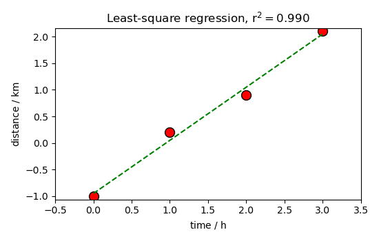
<_Axes: title={'center': 'Least-square regression, $r^2=0.990$'}, xlabel='time $\\mathrm{/\\ \\mathrm{h}}$', ylabel='distance $\\mathrm{/\\ \\mathrm{km}}$'>

This ends the example ! The following line can be uncommented if no plot shows when running the .py script

scp.show()