MCR-ALS with kinetic constraints

In this example, we perform the MCR ALS optimization of the UV-vis of spectra resulting from a three-component reaction A -> B -> C which was investigated by UV–Vis spectroscopy. Full details on the reaction and data acquisition conditions can be found in Bijlsma et al. [2001] . The data can be downloded from the author website Biosystems Data Analysis group University of Amsterdam (Copyright 2005 Biosystems Data Analysis Group ; Universiteit van Amsterdam )

import numpy as np

import spectrochempy as scp

Loading a NDDataset

DownLoad the data at (Kinetic data set (UV-VIS) ) using the read function.

data = scp.read("http://www.bdagroup.nl/content/Downloads/datasets/18_sb_uv_vis.zip")

For sake of demonstration, we will focus on a single run. For example, we extract only the data for the run #9 (dataset name: 'x9b' ).

Let’s search it. Data is a list of pairs of NDDataset, a pair of each run. The name we are looking for is the name of the second dataset in a apir.

for pair in data:
    if pair[1].name == "x9b":
        ds = pair
        break

now we have the required pair of dataset.

The first dataset incontains the time in seconds since the start of the reaction (t=0). The first column of the matrix contains the wavelength axis and the remaining columns are the measured UV-VIS spectra (wavelengths x timepoints)

print("\n NDDataset names: " + str([d.name for d in ds]))

NDDataset names: ['RelTime', 'x9b']

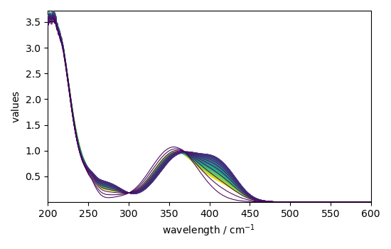
We load the experimental spectra (in ds[1]), add the y (time) and x (wavelength) coordinates, and keep one spectrum of out 4:

D = scp.NDDataset(ds[1][:, 1:].data.T)
D.y = scp.Coord(ds[0].data.squeeze(), title="time") / 60
D.x = scp.Coord(ds[1][:, 0].data.squeeze(), title="wavelength / cm$^{-1}$")
D = D[::4]
_ = D.plot()

A first estimate of the concentrations can be obtained by EFA:

print("compute EFA...")
efa = scp.EFA()
efa.fit(D[:, 300.0:500.0])
efa.n_components = 3
C0 = efa.transform()
C0 = C0 / C0.max(dim="y") * 5.0
_ = C0.T.plot()

compute EFA...

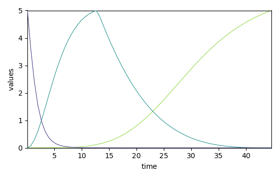
We can get a better estimate of the concentration (C) and pure spectra profiles (St) by soft MCR-ALS:

mcr_1 = scp.MCRALS(log_level="INFO")
_ = mcr_1.fit(D, C0)

_ = mcr_1.C.T.plot()
_ = mcr_1.St.plot()

• 
• 

Concentration profile initialized with 3 components
Initial spectra profile computed
***           ALS optimisation log            ***
#iter     RSE / PCA        RSE / Exp      %change
-------------------------------------------------
  1        0.002813        0.005863      -99.286895
  2        0.002810        0.005861       -0.020846
converged !

Kinetic constraints can be added, i.e., imposing that the concentration profiles obey a kinetic model. To do so we first define an ActionMAssKinetics object with roughly estimated rate constants:

reactions = ("A -> B", "B -> C")
species_concentrations = {"A": 5.0, "B": 0.0, "C": 0.0}
k0 = np.array((0.5, 0.05))
kin = scp.ActionMassKinetics(reactions, species_concentrations, k0)

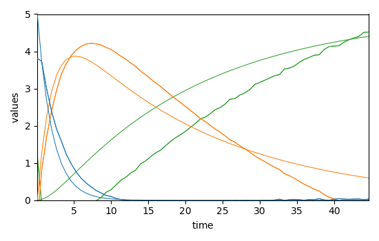
The concentration profile obtained with this approximate model can be computed and compared with those of the soft MCR-ALS:

Ckin = kin.integrate(D.y.data)
_ = mcr_1.C.T.plot(linestyle="-", cmap=None)
_ = Ckin.T.plot(clear=False, cmap=None)

Even though very approximate, the same values can be used to run a hard-soft MCR-ALS:

X = D[:, 300.0:500.0]
param_to_optimize = {"k[0]": 0.5, "k[1]": 0.05}
mcr_2 = scp.MCRALS()
mcr_2.hardConc = [0, 1, 2]
mcr_2.getConc = kin.fit_to_concentrations
mcr_2.argsGetConc = ([0, 1, 2], [0, 1, 2], param_to_optimize)
mcr_2.kwargsGetConc = {"ivp_solver_kwargs": {"return_NDDataset": False}}

mcr_2.fit(X, Ckin)

Optimization of the parameters.
         Initial parameters: [     0.5     0.05]
         Initial function value: 6.457764
Optimization terminated successfully.
         Current function value: 4.313287
         Iterations: 28
         Function evaluations: 54
         Optimization time: 0:00:00.140123
         Final parameters: [  0.3975  0.05019]
Optimization of the parameters.
         Initial parameters: [  0.3975  0.05019]
         Initial function value: 3.465589
Optimization terminated successfully.
         Current function value: 2.678511
         Iterations: 24
         Function evaluations: 48
         Optimization time: 0:00:00.118559
         Final parameters: [  0.3507  0.05016]
Optimization of the parameters.
         Initial parameters: [  0.3507  0.05016]
         Initial function value: 2.257758
Optimization terminated successfully.
         Current function value: 1.901765
         Iterations: 23
         Function evaluations: 46
         Optimization time: 0:00:00.109222
         Final parameters: [  0.3244  0.05001]
Optimization of the parameters.
         Initial parameters: [  0.3244  0.05001]
         Initial function value: 1.665581
Optimization terminated successfully.
         Current function value: 1.482184
         Iterations: 19
         Function evaluations: 39
         Optimization time: 0:00:00.090787
         Final parameters: [  0.3079   0.0498]

<spectrochempy.analysis.mcrals.MCRALS object at 0x7f15afba6580>

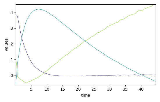
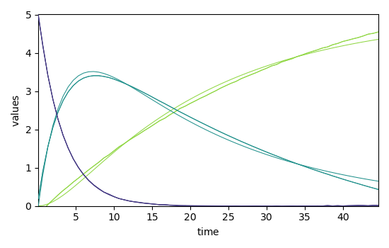
Now, let's compare the concentration profile of MCR-ALS (C = X(C$_{kin}^+$ X)$^+$) with that of the optimized kinetic model (C$_{kin}$ equiv$ C_constrained):

# sphinx_gallery_thumbnail_number = 6

_ = mcr_2.C.T.plot()
_ = mcr_2.C_constrained.T.plot(clear=False)

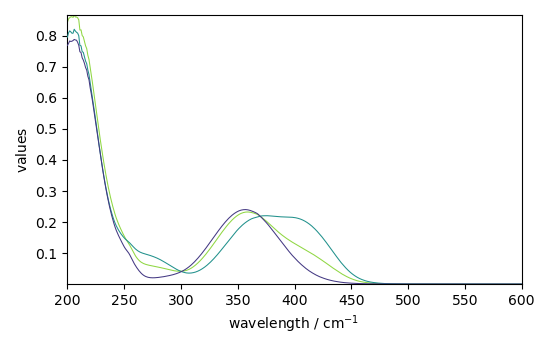
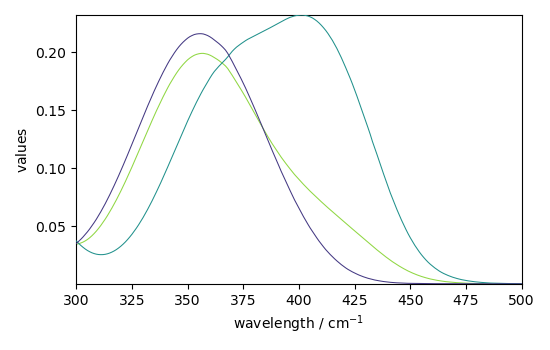
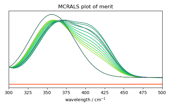
Finally, let's plot some of the pure spectra profiles St, and the

reconstructed dataset (X_hat = C St) vs original dataset (X) and residuals.

_ = mcr_2.St.plot()
_ = mcr_2.plotmerit(nb_traces=10)

• 
• 

This ends the example ! The following line can be uncommented if no plot shows when running the .py script

# scp.show()