Warning

You are reading the documentation related to the development version. Go here if you are looking for the documentation of the stable release.

spectrochempy.IRIS¶

class IRIS(log_level='WARNING', warm_start=False, *, qpsolver='osqp', reg_par=None)[source]¶

Integral inversion solver for spectroscopic data (IRIS).

IRIS, a model developed by Stelmachowski et al. [2013], solves integral equation of the first kind of 1 or 2 dimensions, i.e., finds a distribution function \(f(p)\) or \(f(c,p)\) of contributions to univariate data \(a(p)\) or multivariate \(a(c, p)\) data evolving with an external experimental variable \(p\) (time, pressure, temperature, concentration, …) according to the integral transform:

\[a(c, p) = \int_{min}^{max} k(q, p) f(c, q) dq\]

\[a(p) = \int_{min}^{max} k(q, p) f(q) dq\]

where the kernel \(k(q, p)\) expresses the functional dependence of a single contribution with respect to the experimental variable \(p\) and ‘internal’ physico-chemical variable \(q\) .

Regularization is triggered when reg_par is set to an array of two or three values.

If reg_par has two values [min, max], the optimum regularization parameter is searched between \(10^{min}\) and \(10^{max}\). Automatic search of the regularization is made using the Cultrera_Callegaro algorithm (:cite:p:cultrera:2020) which involves the Menger curvature of a circumcircle and the golden section search method.

If three values are given ([min, max, num]), then the inversion will be made for num values evenly spaced on a log scale between \(10^{min}\) and \(10^{max}\).

Parameters

log_level (any of ["INFO", "DEBUG", "WARNING", "ERROR"], optional, default: "WARNING") – The log level at startup. It can be changed later on using the set_log_level method or by changing the log_level attribute.
warm_start (bool, optional, default: False) – When fitting repeatedly on the same dataset, but for multiple parameter values (such as to find the value maximizing performance), it may be possible to reuse previous model learned from the previous parameter value, saving time.

When warm_start is True, the existing fitted model attributes is used to initialize the new model in a subsequent call to fit.
qpsolver (any value of [ 'osqp' , 'quadprog' ], optional, default: 'osqp') – Quatratic programming solver (osqp (default) or quadprog). Note that quadprog is not installed with spectrochempy.
reg_par (list, optional, default: []) – Regularization parameter (two values [ min, max] or three values [ start, stop, num]. If reg_par is None, no regularization is applied.

See also

EFA: Perform an Evolving Factor Analysis (forward and reverse).
FastICA: Perform Independent Component Analysis with a fast algorithm.
MCRALS: Perform MCR-ALS of a dataset knowing the initial \(C\) or \(S^T\) matrix.
NMF: Non-Negative Matrix Factorization.
PCA: Perform Principal Components Analysis.
SIMPLISMA: SIMPLe to use Interactive Self-modeling Mixture Analysis.
SVD: Perform a Singular Value Decomposition.

Attributes Summary

`X`	Return the X input dataset (eventually modified by the model).
`Y`	The `Y` input.
`components`	`NDDataset` with components in feature space (n_components, n_features).
`config`	`traitlets.config.Config` object.
`log`	Return `log` output.
`n_components`	Number of components that were fitted.
`name`	Object name
`qpsolver`	Quatratic programming solver (`osqp` (default) or `quadprog`).
`reg_par`	Regularization parameter (two values [ `min`, `max`] or three values [ `start`, `stop`, `num`].

Methods Summary

`fit`(X[, Y])	Fit the model with `X` as input dataset.
`fit_transform`(X[, Y])	Fit the model with `X` and apply the dimensionality reduction on `X`.
`get_components`([n_components])	Return the component's dataset: (selected n_components, n_features).
`inverse_transform`()	Transform data back to the original space.
`parameters`([replace, removed, default])	Alias for `params` method.
`params`([default])	Current or default configuration values.
`plotdistribution`([index])	Plot the distribution function.
`plotlcurve`([scale, title])	Plot the `L-Curve`.
`plotmerit`([index])	Plot the input dataset, reconstructed dataset and residuals.
`reconstruct`([X_transform])	Transform data back to its original space.
`reduce`([X])	Apply dimensionality reduction to `X`.
`reset`()	Reset configuration parameters to their default values
`to_dict`()	Return config value in a dict form.
`transform`([X])	Apply dimensionality reduction to `X`.

Attributes Documentation

X¶: Return the X input dataset (eventually modified by the model).

Y¶: The Y input.

components¶

NDDataset with components in feature space (n_components, n_features).

See also

get_components: Retrieve only the specified number of components.

config¶: traitlets.config.Config object.

log¶: Return log output.

n_components¶: Number of components that were fitted.

name¶: Object name

qpsolver¶: Quatratic programming solver (osqp (default) or quadprog). Note that quadprog is not installed with spectrochempy.

reg_par¶: Regularization parameter (two values [ min, max] or three values [ start, stop, num]. If reg_par is None, no regularization is applied.

Methods Documentation

fit(X, Y=None)[source]¶

Fit the model with X as input dataset.

Parameters

X (NDDataset or array-like of shape (n_observations, n_features)) – Training data.
Y (any) – Depends on the model.

Returns

self – The fitted instance itself.

See also

fit_transform: Fit the model with an input dataset X and apply the dimensionality reduction on X.
fit_reduce: Alias of fit_transform (Deprecated).

fit_transform(X, Y=None, **kwargs)[source]¶

Fit the model with X and apply the dimensionality reduction on X.

Parameters

X (NDDataset or array-like of shape (n_observations, n_features)) – Training data.
Y (any) – Depends on the model.
**kwargs (keyword parameters, optional) – See Other Parameters.

Returns

NDDataset – Dataset with shape (n_observations, n_components).

Other Parameters

n_components (int, optional) – The number of components to use for the reduction. If not given the number of components is eventually the one specified or determined in the fit process.

get_components(n_components=None)¶

Return the component’s dataset: (selected n_components, n_features).

Parameters: n_components (int, optional, default: None) – The number of components to keep in the output dataset. If None, all calculated components are returned.
Returns: NDDataset – Dataset with shape (n_components, n_features)

inverse_transform()[source]¶

Transform data back to the original space.

The following matrix operation is performed : \(\hat{X} = K.f[i]\) for each value of the regularization parameter.

Returns: NDDataset – The reconstructed dataset.

parameters(replace="params", removed="0.7.1") def parameters(self, default=False)[source]¶: Alias for params method.

params(default=False)[source]¶

Current or default configuration values.

Parameters: default (bool, optional, default: False) – If default is True, the default parameters are returned, else the current values.
Returns: dict – Current or default configuration values.

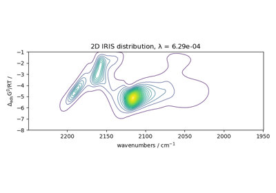
plotdistribution(index=None, **kwargs)[source]¶

Plot the distribution function.

This function plots the distribution function f of the IRIS object.

Parameters

index (int , list or tuple of int, optional, default: None) – Index(es) of the inversions (i.e. of the regularization parameter) to consider. If None, plots for all indices.
**kwargs – Other optional arguments are passed in the plots.

Returns

list of Axes – Subplots.

plotlcurve(scale='ll', title='L curve')[source]¶

Plot the L-Curve.

Parameters

scale (str, optional, default: 'll') – String of 2 letters among 'l'(log) or 'n'(non-log) indicating whether the y and x axes should be log scales.
title (str, optional, default: 'L-curve') – Plot title.

Returns

Axes – The matplotlib axe.

plotmerit(index=None, **kwargs)[source]¶

Plot the input dataset, reconstructed dataset and residuals.

Parameters

index (int, list or tuple of int, optional, default: None) – Index(es) of the inversions (i.e., of the lambda values) to consider. If None plots for all indices.
**kwargs (keyword parameters, optional) – See Other Parameters.

Returns

list of Axes – Subplots.

Other Parameters

colors (tuple or ndarray of 3 colors, optional) – Colors for X , X_hat and residuals E . in the case of 2D, The default colormap is used for X . By default, the three colors are NBlue , NGreen and NRed (which are colorblind friendly).
offset (float, optional, default: None) – Specify the separation (in percent) between the \(X\) , \(X_hat\) and \(E\).
nb_traces (int or 'all', optional) – Number of lines to display. Default is 'all'.
**others (Other keywords parameters) – Parameters passed to the internal plot method of the X dataset.

reconstruct(X_transform=None, **kwargs)[source]¶

Transform data back to its original space.

In other words, return an input X_original whose reduce/transform would be X_transform.

Parameters

X_transform (array-like of shape (n_observations, n_components), optional) – Reduced X data, where n_observations is the number of observations and n_components is the number of components. If X_transform is not provided, a transform of X provided in fit is performed first.
**kwargs (keyword parameters, optional) – See Other Parameters.

Returns

NDDataset – Dataset with shape (n_observations, n_features).

Other Parameters

n_components (int, optional) – The number of components to use for the reduction. If not given the number of components is eventually the one specified or determined in the fit process.

See also

reconstruct: Alias of inverse_transform (Deprecated).

Notes

Deprecated in version 0.6.

reduce(X=None, **kwargs)[source]¶

Apply dimensionality reduction to X.

Parameters

X (NDDataset or array-like of shape (n_observations, n_features), optional) – New data, where n_observations is the number of observations and n_features is the number of features. if not provided, the input dataset of the fit method will be used.
**kwargs (keyword parameters, optional) – See Other Parameters.

Returns

NDDataset – Dataset with shape (n_observations, n_components).

Other Parameters

n_components (int, optional) – The number of components to use for the reduction. If not given the number of components is eventually the one specified or determined in the fit process.

Notes

Deprecated in version 0.6.

reset()[source]¶: Reset configuration parameters to their default values

to_dict()[source]¶

Return config value in a dict form.

Returns: dict – A regular dictionary.

transform(X=None, **kwargs)¶

Apply dimensionality reduction to X.

Parameters

X (NDDataset or array-like of shape (n_observations, n_features), optional) – New data, where n_observations is the number of observations and n_features is the number of features. if not provided, the input dataset of the fit method will be used.
**kwargs (keyword parameters, optional) – See Other Parameters.

Returns

NDDataset – Dataset with shape (n_observations, n_components).

Other Parameters

n_components (int, optional) – The number of components to use for the reduction. If not given the number of components is eventually the one specified or determined in the fit process.

Examples using spectrochempy.IRIS

2D-IRIS analysis example