NDDataset coordinates example

In this example, we show how coordinates can be used in SpectroChemPy

import spectrochempy as scp

Uploading a dataset

X = scp.read("irdata/CO@Mo_Al2O3.SPG")

X has two coordinates: * wavenumbers named “x” * and timestamps (i.e., the time of recording) named “y”.

print(X.coordset)

CoordSet: [x:wavenumbers, y:acquisition timestamp (GMT)]

To display them individually use the x and y attributes of the dataset X:

X.x

size	3112
title	wavenumbers
coordinates	[ 4000 3999 ... 1001 999.9] cm⁻¹

X.y

size	19
title	acquisition timestamp (GMT)
coordinates	[1.477e+09 1.477e+09 ... 1.477e+09 1.477e+09] s
labels	[[ 2016-10-18 13:49:35+00:00 2016-10-18 13:54:06+00:00 ... 2016-10-18 16:01:33+00:00 2016-10-18 16:06:37+00:00] [ *Résultat de Soustraction:04_Mo_Al2O3_calc_0.003torr_LT_after sulf_Oct 18 15:46:42 2016 (GMT+02:00) *Résultat de Soustraction:04_Mo_Al2O3_calc_0.004torr_LT_after sulf_Oct 18 15:51:12 2016 (GMT+02:00) ... *Résultat de Soustraction:04_Mo_Al2O3_calc_0.905torr_LT_after sulf_Oct 18 17:58:42 2016 (GMT+02:00) *Résultat de Soustraction:04_Mo_Al2O3_calc_1.004torr_LT_after sulf_Oct 18 18:03:41 2016 (GMT+02:00)]]

Setting new coordinates

In this example, each experiment have a timestamp corresponds to the time when a given pressure of CO in the infrared cell was set.

Hence, it would be interesting to replace the “useless” timestamps (y ) by a pressure coordinates:

pressures = [
    0.00300,
    0.00400,
    0.00900,
    0.01400,
    0.02100,
    0.02600,
    0.03600,
    0.05100,
    0.09300,
    0.15000,
    0.20300,
    0.30000,
    0.40400,
    0.50300,
    0.60200,
    0.70200,
    0.80100,
    0.90500,
    1.00400,
]

1. A first way to do this is to replace the time coordinates by the pressure coordinate

(we first make a copy of the time coordinates for later use the original will be destroyed by the following operation)

c_times = X.y.copy()

Now we perform the replacement with this new coordinate:

c_pressures = scp.Coord(pressures, title="pressure", units="torr")
X.y = c_pressures
print(X.y)

Coord: [float64] torr (size: 19)

2. A second way is to affect several coordinates to the corresponding dimension. To do this, the simplest is to affect a list of coordinates instead of a single one:

X.y = [c_times, c_pressures]
print(X.y)

CoordSet: [_1:acquisition timestamp (GMT), _2:pressure]

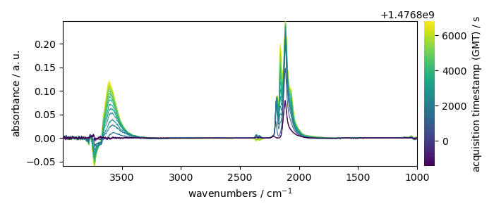
By default, the current coordinate is the first one (here c_times ). For example, it will be used for plotting:

prefs = X.preferences
prefs.figure.figsize = (7, 3)
_ = X.plot(colorbar=True)
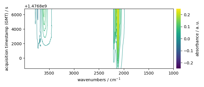
_ = X.plot_map(colorbar=True)

• 
• 

To seamlessly work with the second coordinates (pressures), we can change the default coordinate:

X.y.select(2)  # to select coordinate `_2`
X.y.default

size	19
title	pressure
coordinates	[ 0.003 0.004 ... 0.905 1.004] torr

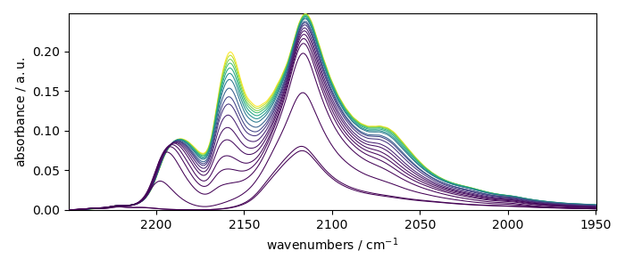
Let’s now plot the spectral range of interest. The default coordinate is now used:

X_ = X[:, 2250.0:1950.0]
print(X_.y.default)
_ = X_.plot()
_ = X_.plot_map()

• 
• 

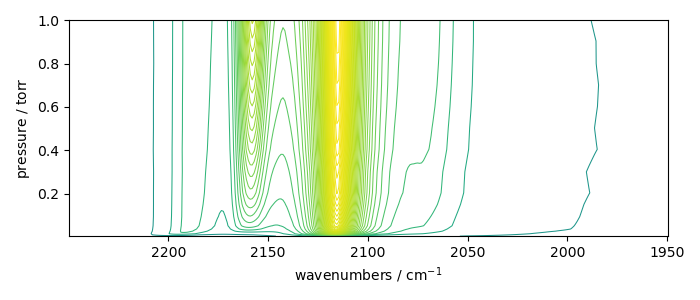
Coord: [float64] torr (size: 19)

The same can be done for the x coordinates.

Let’s take for instance row with index 10 of the previous dataset

row10 = X_[10].squeeze()
row10.plot()
print(row10.coordset)

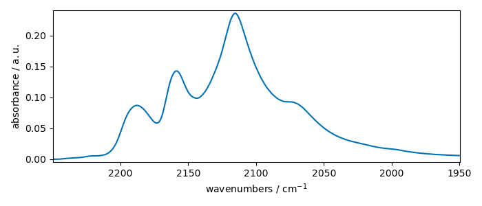
CoordSet: [x:wavenumbers]

Now we wants to add a coordinate with the wavelength instead of wavenumber.

c_wavenumber = row10.x.copy()
c_wavelength = row10.x.to("nanometer")
print(c_wavenumber, c_wavelength)
row10.x = [c_wavenumber, c_wavelength]
row10.x.select(2)
_ = row10.plot()

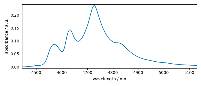
Coord: [float64] cm⁻¹ (size: 312) Coord: [float64] nm (size: 312)

This ends the example ! The following line can be uncommented if no plot shows when running the .py script

scp.show()