Note
Go to the end to download the full example code
Fitting 1D dataset
In this example, we find the least square solution of a simple linear equation.
# sphinx_gallery_thumbnail_number = 2
import os

import spectrochempy as scp
Let’s take an IR spectrum
nd = scp.NDDataset.read_omnic(os.path.join("irdata", "nh4y-activation.spg"))
and select only the OH region:
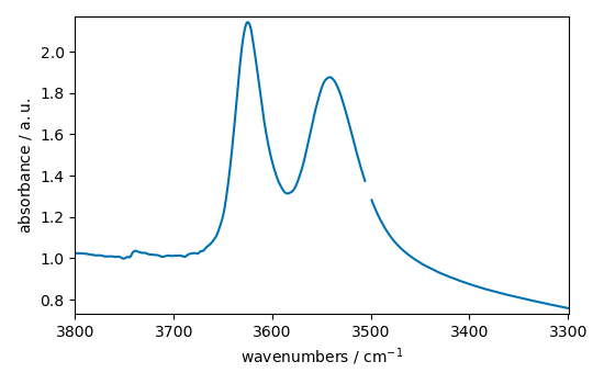
<_Axes: xlabel='wavenumbers $\\mathrm{/\\ \\mathrm{cm}^{-1}}$', ylabel='absorbance $\\mathrm{/\\ \\mathrm{a.u.}}$'>
Perform a Fit Fit parameters are defined in a script (a single text as below)
script = """
#-----------------------------------------------------------
# syntax for parameters definition:
# name: value, low_bound,  high_bound
# available prefix:
#  # for comments
#  * for fixed parameters
#  $ for variable parameters
#  > for reference to a parameter in the COMMON block
#    (> is forbidden in the COMMON block)
# common block parameters should not have a _ in their names
#-----------------------------------------------------------
#

COMMON:
# common parameters ex.
# $ gwidth: 1.0, 0.0, none
$ gratio: 0.1, 0.0, 1.0

MODEL: LINE_1
shape: asymmetricvoigtmodel
    * ampl:  1.1, 0.0, none
    $ pos:   3620, 3400.0, 3700.0
    $ ratio: 0.0147, 0.0, 1.0
    $ asym: 0.1, 0, 1
    $ width: 50, 0, 1000

MODEL: LINE_2
shape: asymmetricvoigtmodel
    $ ampl:  0.8, 0.0, none
    $ pos:   3540, 3400.0, 3700.0
    > ratio: gratio
    $ asym: 0.1, 0, 1
    $ width: 50, 0, 1000

"""
create an Optimize object
f1 = scp.Optimize(log_level="INFO")
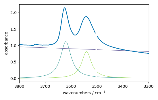
Show plot and the starting model using the dry parameters (of course it is advisable to be as close as possible of a good expectation
f1.script = script

# set dry and continue to show starting model
# reset dry and continue to show starting model
f1.dry = True
f1.autobase = True
f1.fit(ndOH)

# get some information
scp.info_(f"numbers of components: {f1.n_components}")
ndOH.plot()
ax = (f1.components[:]).plot(clear=False)
ax.autoscale(enable=True, axis="y")
 **************************************************
   Entering fitting procedure
 **************************************************


 **************************************************
   Starting parameters:
 **************************************************
 #PARAMETER SCRIPT

COMMON:
        $ gratio:     0.1000, 0.0, 1.0

MODEL: line_1
shape: asymmetricvoigtmodel
        * ampl:     1.1000, 0.0, none
        $ asym:     0.1000, 0, 1
        $ pos:  3620.0000, 3400.0, 3700.0
        $ ratio:     0.0147, 0.0, 1.0
        $ width:    50.0000, 0, 1000

MODEL: line_2
shape: asymmetricvoigtmodel
        $ ampl:     0.8000, 0.0, none
        $ asym:     0.1000, 0, 1
        $ pos:  3540.0000, 3400.0, 3700.0
        > ratio:gratio
        $ width:    50.0000, 0, 1000

 numbers of components: 2
Now perform a fit with maximum 1000 iterations
f1.max_iter = 1000
f1.fit(ndOH)
 **************************************************
   Entering fitting procedure
 **************************************************


 Iterations: 10, Calls: 23 (chi2: 0.95533)


 Iterations: 20, Calls: 34 (chi2: 0.71596)


 Iterations: 30, Calls: 53 (chi2: 0.40984)


 Iterations: 40, Calls: 71 (chi2: 0.39049)


 Iterations: 50, Calls: 86 (chi2: 0.37602)


 Iterations: 60, Calls: 101 (chi2: 0.36717)


 Iterations: 70, Calls: 114 (chi2: 0.35461)


 Iterations: 80, Calls: 132 (chi2: 0.34740)


 Iterations: 90, Calls: 143 (chi2: 0.32942)


 Iterations: 100, Calls: 157 (chi2: 0.32827)


 Iterations: 110, Calls: 171 (chi2: 0.32183)


 Iterations: 120, Calls: 187 (chi2: 0.31899)


 Iterations: 130, Calls: 201 (chi2: 0.31761)


 Iterations: 140, Calls: 217 (chi2: 0.31577)


 Iterations: 150, Calls: 232 (chi2: 0.31479)


 Iterations: 160, Calls: 245 (chi2: 0.31376)


 Iterations: 170, Calls: 256 (chi2: 0.31378)


 Iterations: 180, Calls: 269 (chi2: 0.31390)


 Iterations: 190, Calls: 284 (chi2: 0.31089)


 Iterations: 200, Calls: 298 (chi2: 0.30378)


 Iterations: 210, Calls: 311 (chi2: 0.29820)


 Iterations: 220, Calls: 324 (chi2: 0.27824)


 Iterations: 230, Calls: 338 (chi2: 0.24827)


 Iterations: 240, Calls: 352 (chi2: 0.22682)


 Iterations: 250, Calls: 364 (chi2: 0.19748)


 Iterations: 260, Calls: 377 (chi2: 0.16695)


 Iterations: 270, Calls: 394 (chi2: 0.14808)


 Iterations: 280, Calls: 410 (chi2: 0.12673)


 Iterations: 290, Calls: 423 (chi2: 0.11528)


 Iterations: 300, Calls: 438 (chi2: 0.11136)


 Iterations: 310, Calls: 452 (chi2: 0.09920)


 Iterations: 320, Calls: 464 (chi2: 0.08977)


 Iterations: 330, Calls: 478 (chi2: 0.08859)


 Iterations: 340, Calls: 493 (chi2: 0.08267)


 Iterations: 350, Calls: 508 (chi2: 0.08088)


 Iterations: 360, Calls: 524 (chi2: 0.07706)


 Iterations: 370, Calls: 538 (chi2: 0.07697)


 Iterations: 380, Calls: 550 (chi2: 0.07584)


 Iterations: 390, Calls: 566 (chi2: 0.07506)


 Iterations: 400, Calls: 580 (chi2: 0.07477)


 Iterations: 410, Calls: 596 (chi2: 0.07461)


 Iterations: 420, Calls: 611 (chi2: 0.07455)


 Iterations: 430, Calls: 623 (chi2: 0.07445)


 Iterations: 440, Calls: 637 (chi2: 0.07440)


 Iterations: 450, Calls: 648 (chi2: 0.07417)


 Iterations: 460, Calls: 661 (chi2: 0.07413)


 Iterations: 470, Calls: 674 (chi2: 0.07409)


 Iterations: 480, Calls: 687 (chi2: 0.07391)


 Iterations: 490, Calls: 700 (chi2: 0.07368)


 Iterations: 500, Calls: 713 (chi2: 0.07282)


 Iterations: 510, Calls: 727 (chi2: 0.07150)


 Iterations: 520, Calls: 739 (chi2: 0.07054)


 Iterations: 530, Calls: 754 (chi2: 0.06691)


 Iterations: 540, Calls: 767 (chi2: 0.06623)


 Iterations: 550, Calls: 782 (chi2: 0.06500)


 Iterations: 560, Calls: 796 (chi2: 0.06425)


 Iterations: 570, Calls: 811 (chi2: 0.06396)


 Iterations: 580, Calls: 825 (chi2: 0.06336)


 Iterations: 590, Calls: 838 (chi2: 0.06330)


 Iterations: 600, Calls: 852 (chi2: 0.06278)


 Iterations: 610, Calls: 866 (chi2: 0.06221)


 Iterations: 620, Calls: 881 (chi2: 0.06221)


 Iterations: 630, Calls: 894 (chi2: 0.06097)


 Iterations: 640, Calls: 907 (chi2: 0.05989)


 Iterations: 650, Calls: 920 (chi2: 0.05849)


 Iterations: 660, Calls: 932 (chi2: 0.05741)


 Iterations: 670, Calls: 947 (chi2: 0.05484)


 Iterations: 680, Calls: 959 (chi2: 0.05228)


 Iterations: 690, Calls: 976 (chi2: 0.04946)


 Iterations: 700, Calls: 990 (chi2: 0.04601)


 Iterations: 710, Calls: 1004 (chi2: 0.04244)


 Iterations: 720, Calls: 1017 (chi2: 0.04255)


 Iterations: 730, Calls: 1033 (chi2: 0.04031)


 Iterations: 740, Calls: 1047 (chi2: 0.03897)


 Iterations: 750, Calls: 1059 (chi2: 0.03899)


 Iterations: 760, Calls: 1076 (chi2: 0.03793)


 Iterations: 770, Calls: 1090 (chi2: 0.03799)


 Iterations: 780, Calls: 1104 (chi2: 0.03747)


 Iterations: 790, Calls: 1117 (chi2: 0.03713)


 Iterations: 800, Calls: 1130 (chi2: 0.03707)


 Iterations: 810, Calls: 1143 (chi2: 0.03683)


 Iterations: 820, Calls: 1160 (chi2: 0.03674)


 Iterations: 830, Calls: 1173 (chi2: 0.03667)


 Iterations: 840, Calls: 1189 (chi2: 0.03667)


 Iterations: 850, Calls: 1206 (chi2: 0.03664)


 Iterations: 860, Calls: 1221 (chi2: 0.03664)


 Iterations: 870, Calls: 1238 (chi2: 0.03663)


 Iterations: 880, Calls: 1257 (chi2: 0.03663)


 Iterations: 890, Calls: 1275 (chi2: 0.03663)


 Iterations: 900, Calls: 1292 (chi2: 0.03663)


 Iterations: 910, Calls: 1307 (chi2: 0.03663)


 Iterations: 920, Calls: 1323 (chi2: 0.03663)


 Iterations: 930, Calls: 1338 (chi2: 0.03663)


 Iterations: 940, Calls: 1353 (chi2: 0.03663)


 Iterations: 950, Calls: 1367 (chi2: 0.03663)


 Iterations: 960, Calls: 1380 (chi2: 0.03663)


 Iterations: 970, Calls: 1396 (chi2: 0.03663)


 Iterations: 980, Calls: 1408 (chi2: 0.03663)


 Iterations: 990, Calls: 1420 (chi2: 0.03663)
/home/runner/micromamba-root/envs/scpy/lib/python3.9/site-packages/spectrochempy/application/application.py:782: UserWarning: Maximum number of iterations reached.
  warnings.warn(msg, *args, **kwargs)


 **************************************************
   Result:
 **************************************************
 #PARAMETER SCRIPT

COMMON:
        $ gratio:     0.2943, 0.0, 1.0

MODEL: line_1
shape: asymmetricvoigtmodel
        * ampl:     1.1000, 0.0, none
        $ asym:     0.6383, 0, 1
        $ pos:  3623.5311, 3400.0, 3700.0
        $ ratio:     0.4842, 0.0, 1.0
        $ width:    43.0340, 0, 1000

MODEL: line_2
shape: asymmetricvoigtmodel
        $ ampl:     0.9176, 0.0, none
        $ asym:     0.9734, 0, 1
        $ pos:  3537.1487, 3400.0, 3700.0
        > ratio:gratio
        $ width:    79.2192, 0, 1000


<spectrochempy.analysis.optimize.optimize.Optimize object at 0x7f15afb0ee50>
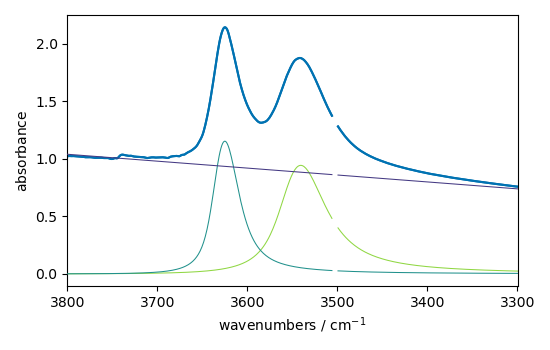
Show the result
ndOH.plot()
ax = (f1.components[:]).plot(clear=False)
ax.autoscale(enable=True, axis="y")

# plotmerit
som = f1.inverse_transform()
f1.plotmerit(ndOH, som, method="scatter", markevery=5, markersize=2)
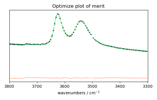
<_Axes: title={'center': 'Optimize plot of merit'}, xlabel='wavenumbers $\\mathrm{/\\ \\mathrm{cm}^{-1}}$', ylabel='absorbance $\\mathrm{/\\ \\mathrm{a.u.}}$'>
This ends the example ! The following line can be uncommented if no plot shows when running the .py script
scp.show()
Total running time of the script: ( 0 minutes 2.346 seconds)