PCA analysis example

In this example, we perform the PCA dimensionality reduction of a spectra dataset

Import the spectrochempy API package

import spectrochempy as scp

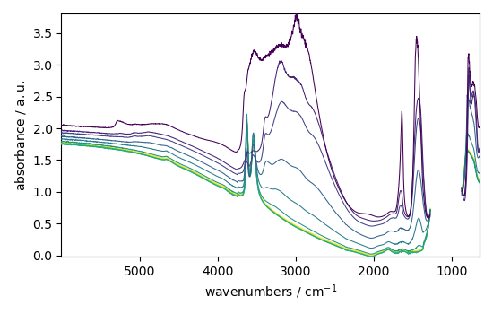
Load a dataset

dataset = scp.read_omnic("irdata/nh4y-activation.spg")[::5]
print(dataset)
_ = dataset.plot()

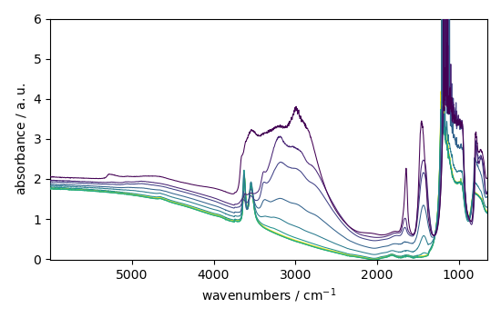
NDDataset: [float64] a.u. (shape: (y:11, x:5549))

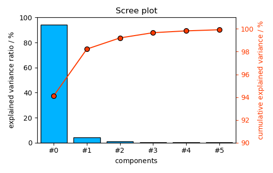
Create a PCA object and fit the dataset so that the explained variance is greater or equal to 99.9%

pca = scp.PCA(n_components=0.999)
pca.fit(dataset)

<spectrochempy.analysis.pca.PCA object at 0x7f15af643b80>

The number of fitted components is given by the n_components attribute (We obtain 23 components)

pca.n_components

6

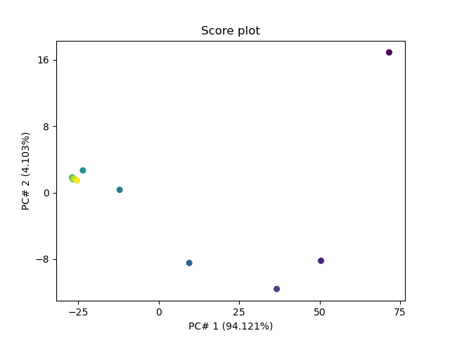
Transform the dataset to a lower dimensionality using all the fitted components

scores = pca.transform()
scores

name	nh4y-activation_PCA.transform
author	runner@fv-az626-878
created	2023-06-06 01:27:26+00:00
history	2023-06-06 01:27:26+00:00> Created using method PCA.transform
DATA
title
values	[[ 71.56 16.87 ... -0.006776 -0.216] [ 50.39 -8.205 ... 0.5566 0.03804] ... [ -26.25 1.694 ... 0.1281 -0.6077] [ -25.46 1.456 ... 4.175 0.7883]]
shape	(y:11, x:6)
DIMENSION `x`
size	6
title	components
labels	[ #0 #1 #2 #3 #4 #5]
DIMENSION `y`
size	11
title	acquisition timestamp (GMT)
coordinates	[1.468e+09 1.468e+09 ... 1.468e+09 1.468e+09] s
labels	[[ 2016-07-06 19:03:14+00:00 2016-07-06 19:53:14+00:00 ... 2016-07-07 02:43:15+00:00 2016-07-07 03:33:17+00:00] [ vz0466.spa, Wed Jul 06 21:00:38 2016 (GMT+02:00) vz0471.spa, Wed Jul 06 21:50:37 2016 (GMT+02:00) ... vz0512.spa, Thu Jul 07 04:40:39 2016 (GMT+02:00) vz0517.spa, Thu Jul 07 05:30:41 2016 (GMT+02:00)]]

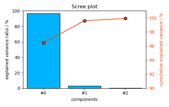
Finally, display the results graphically ScreePlot

_ = pca.screeplot()

• 
• 

Score Plot

_ = pca.scoreplot(scores, 1, 2)

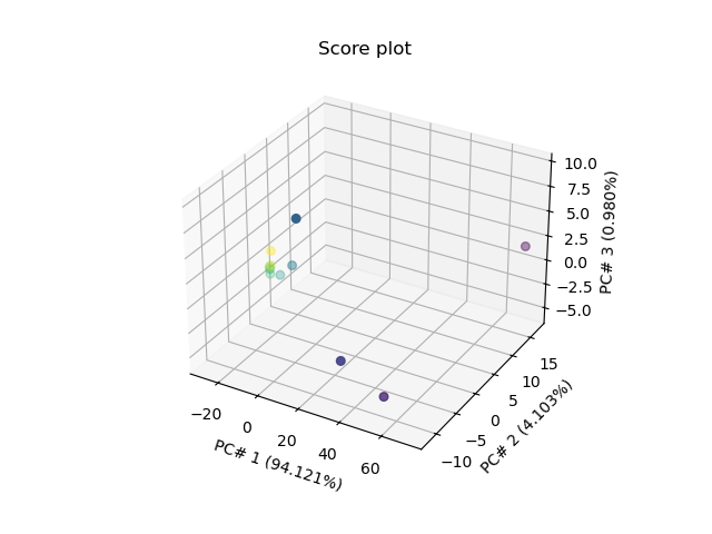
Score Plot for 3 PC’s in 3D

_ = pca.scoreplot(scores, 1, 2, 3)

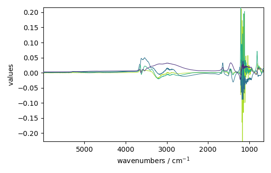
Displays 4 loadings

_ = pca.loadings[:4].plot(legend=True)

Here we do a masking of the saturated region between 882 and 1280 cm^-1

dataset[
    :, 882.0:1280.0
] = scp.MASKED  # remember: use float numbers for slicing (not integer)
_ = dataset.plot()

Apply the PCA model

pca = scp.PCA(n_components=0.999)
pca.fit(dataset)
pca.n_components

3

As seen above, now only 4 components instead of 23 are necessary to 99.9% of explained variance.

_ = pca.screeplot()

• 
• 

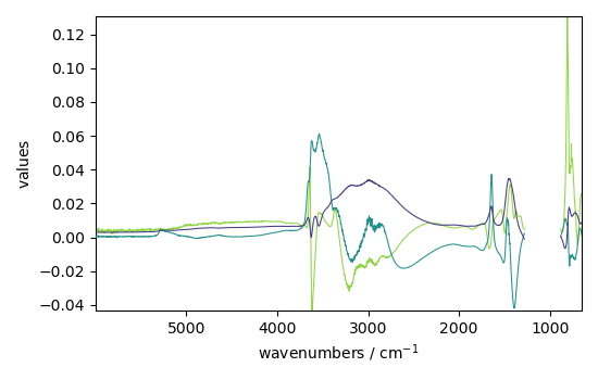
Displays the loadings

_ = pca.loadings.plot(legend=True)

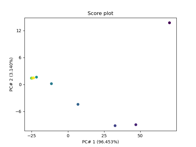
Let’s plot the scores

scores = pca.transform()
_ = pca.scoreplot(scores, 1, 2)

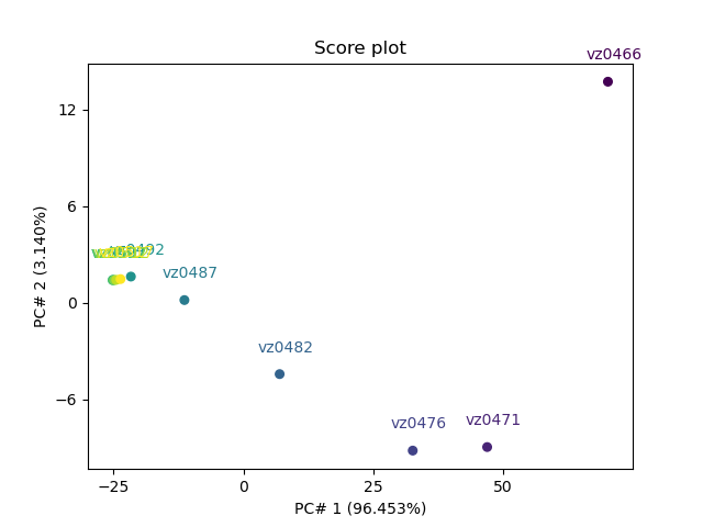
Our dataset has already two columns of labels for the spectra but there are little too long for display on plots.

scores.y.labels

array([[  2016-07-06 19:03:14+00:00,   vz0466.spa, Wed Jul 06 21:00:38 2016 (GMT+02:00)],
       [  2016-07-06 19:53:14+00:00,   vz0471.spa, Wed Jul 06 21:50:37 2016 (GMT+02:00)],
       ...,
       [  2016-07-07 02:43:15+00:00,   vz0512.spa, Thu Jul 07 04:40:39 2016 (GMT+02:00)],
       [  2016-07-07 03:33:17+00:00,   vz0517.spa, Thu Jul 07 05:30:41 2016 (GMT+02:00)]], dtype=object)

So we define some short labels for each component, and add them as a third column:

labels = [lab[:6] for lab in dataset.y.labels[:, 1]]
scores.y.labels = labels  # Note this does not replace previous labels,
# but adds a column.

now display thse

_ = pca.scoreplot(scores, 1, 2, show_labels=True, labels_column=2)

This ends the example ! The following line can be uncommented if no plot shows when running the .py script

# scp.show()