SIMPLISMA example

In this example, we perform the PCA dimensionality reduction of a spectra dataset

Import the spectrochempy API package (and the SIMPLISMA model independently)

import spectrochempy as scp

Load a matlab datasets

print("Dataset (Jaumot et al., Chemometr. Intell. Lab. 76 (2005) 101-110)):")
lnd = scp.read_matlab("matlabdata/als2004dataset.MAT", merge=False)
for mat in lnd:
    print("    " + mat.name, str(mat.shape))

ds = lnd[-1]
_ = ds.plot()

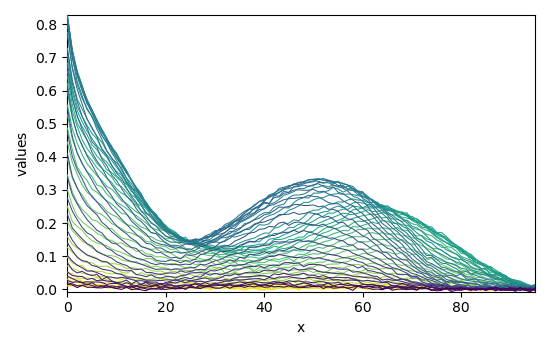
Dataset (Jaumot et al., Chemometr. Intell. Lab. 76 (2005) 101-110)):
    cpure (204, 4)
    MATRIX (204, 96)
    isp_matrix (4, 4)
    spure (4, 96)
    csel_matrix (51, 4)
    m1 (51, 96)

Add some metadata for a nicer display

ds.title = "absorbance"
ds.units = "absorbance"
ds.set_coordset(None, None)
ds.y.title = "elution time"
ds.x.title = "wavelength"
ds.y.units = "hours"
ds.x.units = "nm"

Fit the SIMPLISMA model

print("Fit SIMPLISMA on {}\n".format(ds.name))
simpl = scp.SIMPLISMA(max_components=20, tol=0.2, noise=3, log_level="INFO")
simpl.fit(ds)

Fit SIMPLISMA on m1

/home/runner/micromamba-root/envs/scpy/lib/python3.9/site-packages/spectrochempy/utils/decorators.py:85: DeprecationWarning:  The `max_components` attribute is now deprecated. Use `n_components` instead. `max_components` attribute will be removed in version 0.7.
  warn(
/home/runner/micromamba-root/envs/scpy/lib/python3.9/site-packages/spectrochempy/analysis/simplisma.py:190: UserWarning: SIMPLISMA does not handle easily negative values.
  warn("SIMPLISMA does not handle easily negative values.")

<spectrochempy.analysis.simplisma.SIMPLISMA object at 0x7f15af9543d0>

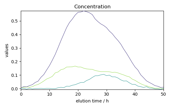
Plot concentration

_ = simpl.C.T.plot(title="Concentration")

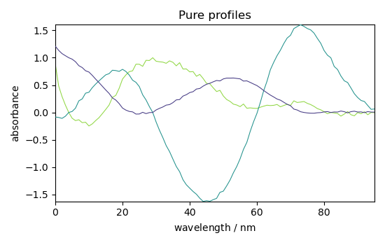
Plot components (St)

# sphinx_gallery_thumbnail_number = 3

_ = simpl.components.plot(title="Pure profiles")

Show the plot of merit after reconstruction oto the original data space

simpl.plotmerit(offset=0, nb_traces=5)

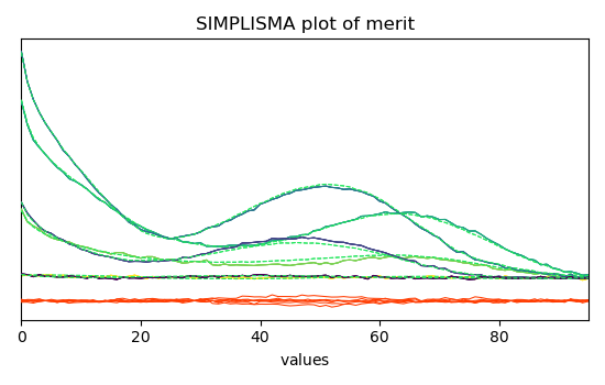
<_Axes: title={'center': 'SIMPLISMA plot of merit'}, xlabel='values $\\mathrm{}$', ylabel='absorbance $\\mathrm{/\\ \\mathrm{a.u.}}$'>

This ends the example ! The following line can be uncommented if no plot shows when running the .py script

# scp.show()