Warning

You are reading the documentation related to the development version. Go here if you are looking for the documentation of the stable release.

EFA example

In this example, we perform the Evolving Factor Analysis

sphinx_gallery_thumbnail_number = 2

import os

import spectrochempy as scp

Upload and preprocess a dataset

datadir = scp.preferences.datadir
dataset = scp.read_omnic(os.path.join(datadir, "irdata", "nh4y-activation.spg"))

Change the time origin

dataset.y -= dataset.y[0]

columns masking

dataset[:, 1230.0:920.0] = scp.MASKED  # do not forget to use float in slicing
dataset[:, 5997.0:5993.0] = scp.MASKED

difference spectra dataset -= dataset[-1]

dataset.plot_stack(title="NH4_Y activation dataset")

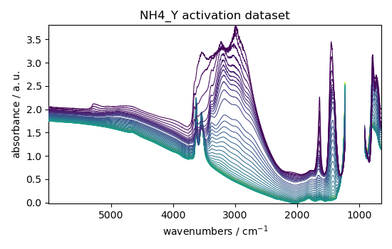
<_Axes: title={'center': 'NH4_Y activation dataset'}, xlabel='wavenumbers $\\mathrm{/\\ \\mathrm{cm}^{-1}}$', ylabel='absorbance $\\mathrm{/\\ \\mathrm{a.u.}}$'>

Evolving Factor Analysis

efa1 = scp.EFA()
_ = efa1.fit(dataset)

Forward evolution of the 5 first components

f = efa1.f_ev[:, :5]
f.T.plot(yscale="log", legend=f.k.labels)

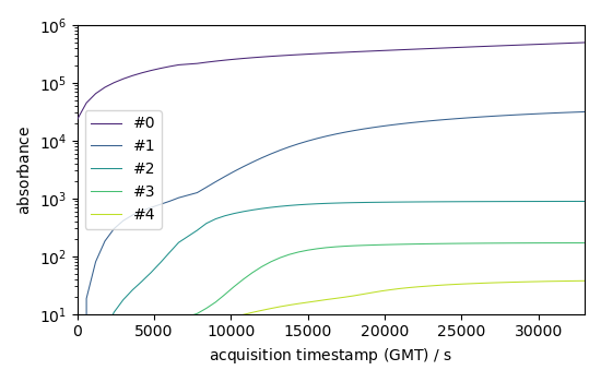
<_Axes: xlabel='acquisition timestamp (GMT) $\\mathrm{/\\ \\mathrm{s}}$', ylabel='absorbance $\\mathrm{}$'>

Note the use of coordinate ‘k’ (component axis) in the expression above. Remember taht to find the actul names of the coordinates, the dims attribute can be used as in the following:

f.dims

# Backward evolution
b = efa1.b_ev[:, :5]
b.T[:5].plot(yscale="log", legend=b.k.labels)

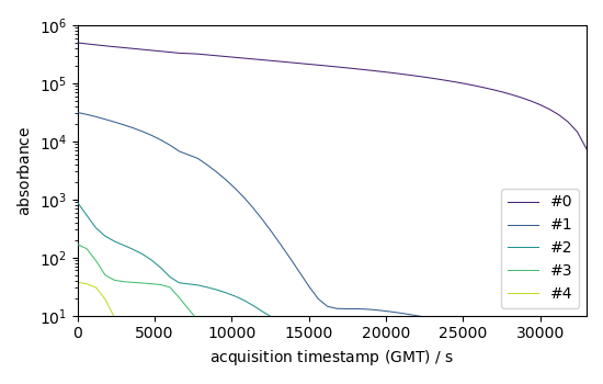
<_Axes: xlabel='acquisition timestamp (GMT) $\\mathrm{/\\ \\mathrm{s}}$', ylabel='absorbance $\\mathrm{}$'>

Show results with 3 components (which seems to already explain a large part of the dataset) we use the magnitude of the 4th component for the cut-off value (assuming it corresponds mostly to noise)

efa1.n_components = 3
efa1.cutoff = efa1.f_ev[:, 3].max()

# get concentration
C1 = efa1.transform()
C1.T.plot(title="EFA determined concentrations", legend=C1.k.labels)

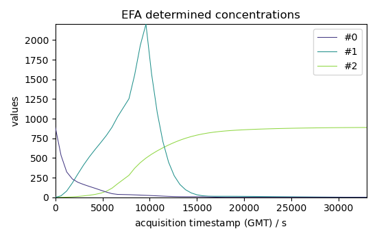
<_Axes: title={'center': 'EFA determined concentrations'}, xlabel='acquisition timestamp (GMT) $\\mathrm{/\\ \\mathrm{s}}$', ylabel='values $\\mathrm{}$'>

Fit transform : Get the concentration in too commands The number of desired components can be passed to the EFA model, followed by the fit_transform method:

efa2 = scp.EFA(n_components=3)
C2 = efa2.fit_transform(dataset)
assert C1 == C2

Get components

St = efa2.get_components()
St.plot(title="components", legend=St.k.labels)

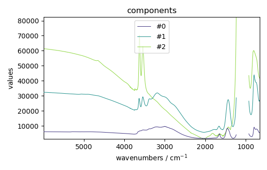
<_Axes: title={'center': 'components'}, xlabel='wavenumbers $\\mathrm{/\\ \\mathrm{cm}^{-1}}$', ylabel='values $\\mathrm{}$'>

Compare with PCA

pca = scp.PCA(n_components=3)
C3 = pca.fit_transform(dataset)

C3.T.plot(title="PCA scores")

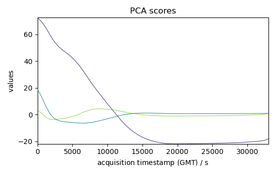
<_Axes: title={'center': 'PCA scores'}, xlabel='acquisition timestamp (GMT) $\\mathrm{/\\ \\mathrm{s}}$', ylabel='values $\\mathrm{}$'>

LT = pca.loadings
LT.plot(title="PCA components", legend=LT.k.labels)

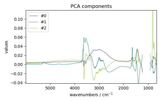
<_Axes: title={'center': 'PCA components'}, xlabel='wavenumbers $\\mathrm{/\\ \\mathrm{cm}^{-1}}$', ylabel='values $\\mathrm{}$'>

This ends the example ! The following line can be uncommented if no plot shows when running the .py script with python

# scp.show()