Note
Go to the end to download the full example code
2D-IRIS analysis example
In this example, we perform the 2D IRIS analysis of CO adsorption on a sulfide catalyst.
import spectrochempy as scp
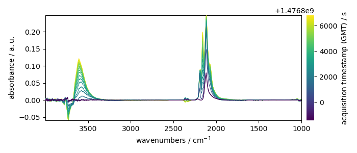
Uploading dataset
X has two coordinates:
* wavenumbers named “x”
* and timestamps (i.e., the time of recording) named “y”.
print(X.coordset)
CoordSet: [x:wavenumbers, y:acquisition timestamp (GMT)]
Setting new coordinates
The y coordinates of the dataset is the acquisition timestamp.
However, each spectrum has been recorded with a given pressure of CO
in the infrared cell.
Hence, it would be interesting to add pressure coordinates to the y dimension:
pressures = [
    0.003,
    0.004,
    0.009,
    0.014,
    0.021,
    0.026,
    0.036,
    0.051,
    0.093,
    0.150,
    0.203,
    0.300,
    0.404,
    0.503,
    0.602,
    0.702,
    0.801,
    0.905,
    1.004,
]

c_pressures = scp.Coord(pressures, title="pressure", units="torr")
Now we can set multiple coordinates:
CoordSet: [_1:acquisition timestamp (GMT), _2:pressure]
To get a detailed a rich display of these coordinates. In a jupyter notebook, just type:
By default, the current coordinate is the first one (here c_times ).
For example, it will be used by default for
plotting:
prefs = X.preferences
prefs.figure.figsize = (7, 3)
_ = X.plot(colorbar=True)
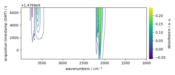
_ = X.plot_map(colorbar=True)
To seamlessly work with the second coordinates (pressures), we can change the default coordinate:
X.y.select(2)  # to select coordinate `_2`
X.y.default
Let’s now plot the spectral range of interest. The default coordinate is now used:
X_ = X[:, 2250.0:1950.0]
print(X_.y.default)
_ = X_.plot()
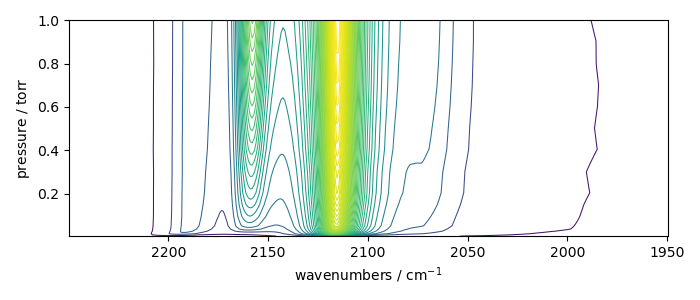
_ = X_.plot_map()
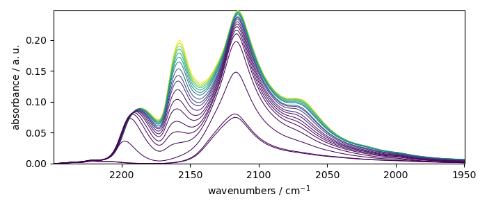
Coord: [float64] torr (size: 19)
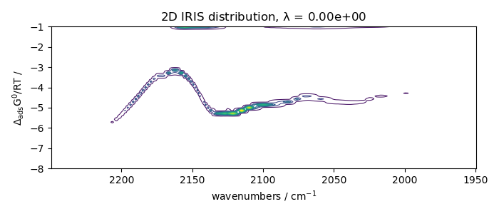
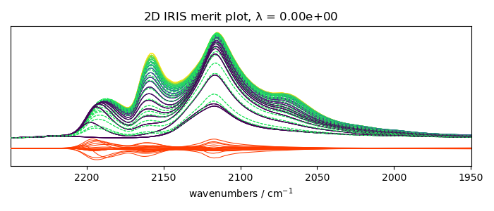
IRIS analysis without regularization
Perform IRIS without regularization (the loglevel can be set to INFO to have
information on the running process)
first we compute the kernel object
K = scp.IrisKernel(X_, "langmuir", q=[-8, -1, 50])
Creating Kernel...
Kernel now ready as IrisKernel().kernel!
The actual kernel is given by the kernel attribute
Now we fit the model - we can pass either the Kernel object or the kernel NDDataset
 Build S matrix (sharpness)
 ... done
 Solving for 312 channels and 19 observations, no regularization
 -->  residuals = 1.09e-01    curvature = 9.14e+04
 Done.

<spectrochempy.analysis.decomposition.iris.IRIS object at 0x7f1a3603a980>
Plots the results
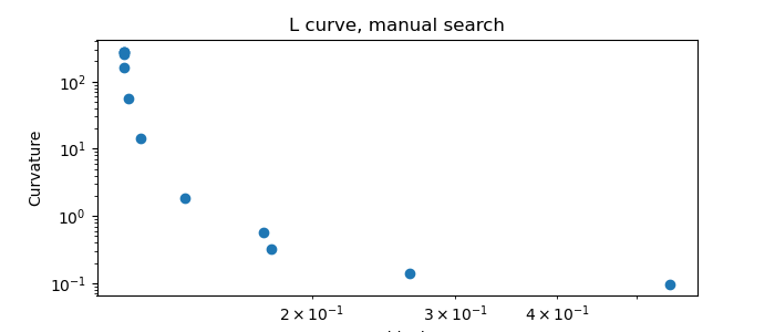
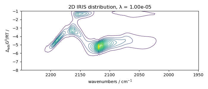
With regularization and a manual search
Perform IRIS with regularization, manual search
We keep the same kernel object as previously - performs the fit.
iris2.fit(X_, K)

iris2.plotlcurve(title="L curve, manual search")
iris2.plotdistribution(-7)
_ = iris2.plotmerit(-7)

Automatic search
%% Now try an automatic search of the regularization parameter:
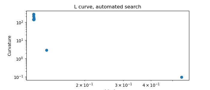
<Axes: title={'center': 'L curve, automated search'}, xlabel='Residuals', ylabel='Curvature'>
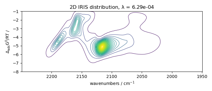
The data corresponding to the largest curvature of the L-curve are at the second last position of output data.
iris3.plotdistribution(-2)
_ = iris3.plotmerit(-2)

This ends the example ! The following line can be uncommented if no plot shows when running the .py script with python
# scp.show()
Total running time of the script: ( 0 minutes 11.779 seconds)