Warning

You are reading the documentation related to the development version. Go here if you are looking for the documentation of the stable release.

FastICA example

Import the spectrochempy API package

import spectrochempy as scp

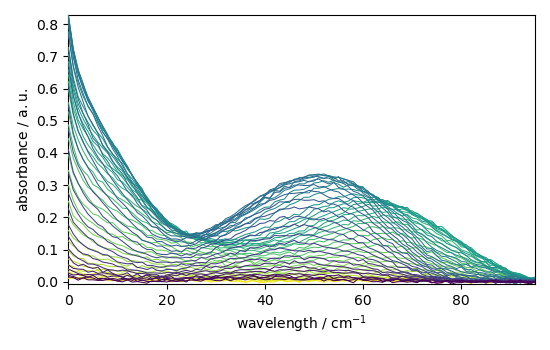
Load, prepare and plot the dataset

Here we use a dataset from Jaumot et al. [2005]

X = scp.read("matlabdata/als2004dataset.MAT")[-1]

X.title = "absorbance"
X.units = "absorbance"
X.set_coordset(None, None)
X.y.title = "elution time"
X.x.title = "wavelength"
X.y.units = "hours"
X.x.units = "cm^-1"
_ = X.plot()

Create and fit a FastICA object

As argument of the object constructor we define log_level to "INFO" to obtain verbose output during fit, and we set the number of component to use at 4.

ica = scp.FastICA(n_components=4)
_ = ica.fit(X)

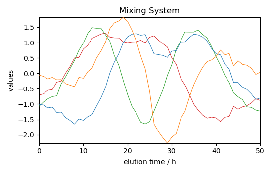
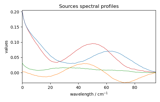
Get the mixing system and source spectral profiles

The mixing system \(A\) and the source spectral profiles \(S^T\) can be obtained as follows (the Sklearn equivalents - also valid with Scpy - are indicated as comments

A = ica.A  # or model.transform()
St = ica.St  # or model.mixing.T

Plot them

_ = A.T.plot(title="Mixing System", colormap=None)
_ = St.plot(title="Sources spectral profiles", colormap=None)

• 
• 

Reconstruct the dataset

The dataset can be reconstructed from these matrices and the mean:

X_hat_a = scp.dot(A, St) + X.mean(dim=0).data
_ = X_hat_a.plot(title=r"$\hat{X} = \bar{X} + A S^t$")

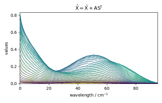
Or using the transform() method:

X_hat_b = ica.inverse_transform()
_ = X_hat_b.plot(title="$\hat{X} =$ ica.inverse_transform()")

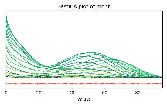
Finally, the quality of the reconstriction can be checked by plotmerit()

_ = ica.plotmerit(nb_traces=15)

This ends the example ! The following line can be uncommented if no plot shows when running the .py script with python

# scp.show()