This is development documentation. Some features are not available in the stable release. View stable documentation.

Build synthetic concentration profiles

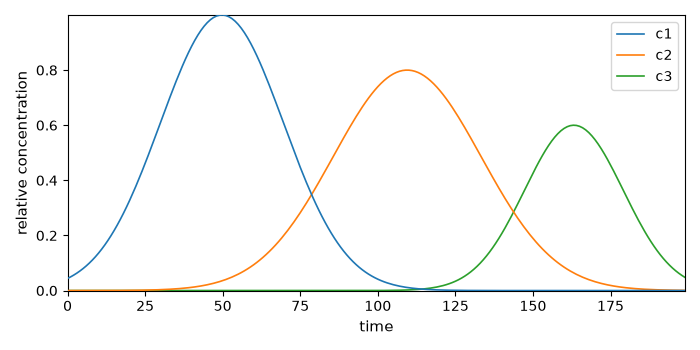
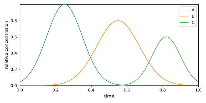
This example shows two convenient ways to build simple synthetic profiles directly with the SpectroChemPy API:

• explicit analytical expressions with top-level math aliases such as scp.exp(...);

• direct line-shape helpers such as scp.gaussian(...) when a built-in model already matches the target profile.

import spectrochempy as scp

Build profiles with analytical expressions

time = scp.linspace(0.0, 1.0, 200)

c1 = scp.exp(-0.5 * ((time - 0.25) / 0.10) ** 2)
c2 = 0.8 * scp.exp(-0.5 * ((time - 0.55) / 0.12) ** 2)
c3 = 0.6 * scp.exp(-0.5 * ((time - 0.82) / 0.08) ** 2)

Assemble as columns of a concentration matrix:

profiles = scp.stack([c1, c2, c3], axis=1)
profiles.x.title = "time"
profiles.y = scp.Coord(labels=["c1", "c2", "c3"], title="species")
profiles.name = "concentrations"
profiles.title = "relative concentration"

ax = profiles.T.plot()
_ = ax.legend()

Use built-in Gaussian line-shape helper

profiles_gaussian = scp.stack(
    [
        scp.gaussian(time, ampl=1.0, pos=0.25, width=0.235, normalized=False),
        scp.gaussian(time, ampl=0.8, pos=0.55, width=0.282, normalized=False),
        scp.gaussian(time, ampl=0.6, pos=0.82, width=0.188, normalized=False),
    ],
    axis=1,
)
profiles_gaussian.x.title = "time"
profiles_gaussian.y = scp.Coord(labels=["A", "B", "C"], title="species")
profiles_gaussian.name = "concentrations_gaussian"
profiles_gaussian.title = "relative concentration"

ax = profiles_gaussian.T.plot()
_ = ax.legend()