Warning

You are reading the documentation related to the development version. Go here if you are looking for the documentation of the stable release.

SpectroChemPy Overview

Welcome to SpectroChemPy! This tutorial will give you a quick overview of the main features and capabilities of the library. We’ll cover:

1. Loading and displaying spectroscopic data

2. Basic data manipulation and plotting

3. Processing techniques (smoothing, baseline correction)

4. Advanced analysis methods

For more detailed information, check out:

• Gallery of Examples

• User’s Guide

• API Reference

Getting Started

First, let’s import SpectroChemPy. By convention, we use the alias scp:

import spectrochempy as scp

SpectroChemPy's API - v.0.7.2.dev7 © Copyright 2014-2025 - A.Travert & C.Fernandez @ LCS

Working with NDDataset Objects

The NDDataset is the core data structure in SpectroChemPy. It’s designed specifically for spectroscopic data and provides:

• Multi-dimensional data support

• Coordinates and units handling

• Built-in visualization

• Processing methods

Let’s load some example FTIR (Fourier Transform Infrared) data:

ds = scp.read("irdata/nh4y-activation.spg")

Exploring Your Data

SpectroChemPy provides multiple ways to inspect your data. Let’s look at:

1. Basic information summary

2. Detailed metadata

# Quick overview
scp.set_loglevel("INFO")  # to see information
scp.info_(ds)

 NDDataset: [float64] a.u. (shape: (y:55, x:5549))

# Detailed information
ds

NDDataset: [float64] a.u. (shape: (y:55, x:5549))[nh4y-activation]

Summary

name

:

nh4y-activation

author

:

runner@fv-az1676-495

created

:

2025-03-02 01:28:15+00:00

description

:

Omnic title: NH4Y-activation.SPG
Omnic filename: /home/runner/.spectrochempy/testdata/irdata/nh4y-activation.spg

history

:

2025-03-02 01:28:15+00:00> Imported from spg file /home/runner/.spectrochempy/testdata/irdata/nh4y-activation.spg.
2025-03-02 01:28:15+00:00> Sorted by date

Data

title

:

absorbance

values

:

...

[[ 2.057 2.061 ... 2.013 2.012]
[ 2.033 2.037 ... 1.913 1.911]
...
[ 1.794 1.791 ... 1.198 1.198]
[ 1.816 1.815 ... 1.24 1.238]] a.u.

shape

:

(y:55, x:5549)

Dimension `x`

size

:

5549

title

:

wavenumbers

coordinates

:

[ 6000 5999 ... 650.9 649.9] cm⁻¹

Dimension `y`

size

:

55

title

:

acquisition timestamp (GMT)

coordinates

:

[1.468e+09 1.468e+09 ... 1.468e+09 1.468e+09] s

labels

:

...

[[ 2016-07-06 19:03:14+00:00 2016-07-06 19:13:14+00:00 ... 2016-07-07 04:03:17+00:00 2016-07-07 04:13:17+00:00]
[ vz0466.spa, Wed Jul 06 21:00:38 2016 (GMT+02:00) vz0467.spa, Wed Jul 06 21:10:38 2016 (GMT+02:00) ...
vz0520.spa, Thu Jul 07 06:00:41 2016 (GMT+02:00) vz0521.spa, Thu Jul 07 06:10:41 2016 (GMT+02:00)]]

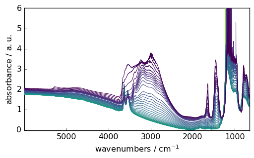
Data Visualization

SpectroChemPy’s plotting capabilities are built on matplotlib but provide spectroscopy-specific features:

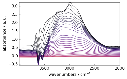
_ = ds.plot()

Data Selection and Manipulation

You can easily select specific regions of your spectra using intuitive slicing. Here we select wavenumbers between 4000 and 2000 cm⁻¹:

region = ds[:, 4000.0:2000.0]
_ = region.plot()

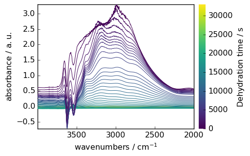
Mathematical Operations

NDDataset supports various mathematical operations. Here’s an example of baseline correction:

# Make y coordinate relative to the first point
region.y -= region.y[0]
region.y.title = "Dehydration time"

# Subtract the last spectrum from all spectra
region -= region[-1]

# Plot with colorbar to show intensity changes
_ = region.plot(colorbar=True)

Data Processing Techniques

SpectroChemPy includes numerous processing methods. Here are some common examples:

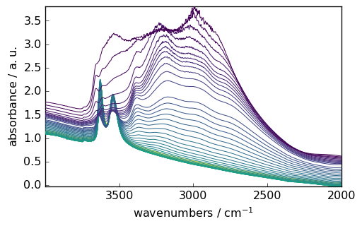
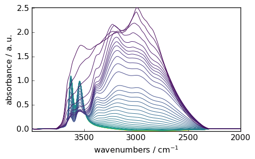
1. Spectral Smoothing

Reduce noise while preserving spectral features:

smoothed = region.smooth(size=51, window="hanning")
_ = smoothed.plot(colormap="magma")

2. Baseline Correction

Remove baseline artifacts using various algorithms:

# Prepare data
region = ds[:, 4000.0:2000.0]
smoothed = region.smooth(size=51, window="hanning")

# Configure baseline correction
blc = scp.Baseline()
blc.ranges = [[2000.0, 2300.0], [3800.0, 3900.0]]  # Baseline regions
blc.multivariate = True
blc.model = "polynomial"
blc.order = "pchip"
blc.n_components = 5

# Apply correction
_ = blc.fit(smoothed)
_ = blc.corrected.plot()

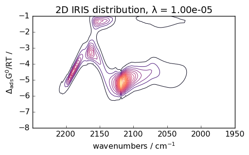
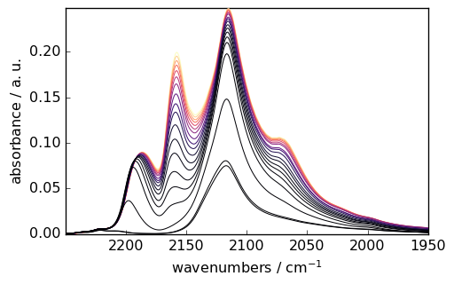
Advanced Analysis as for instance IRIS Processing

IRIS (Iterative Regularized Inverse Solver) is an advanced technique for analyzing spectroscopic data. Here’s an example with CO adsorption data:

# Load and prepare CO adsorption data
ds = scp.read_omnic("irdata/CO@Mo_Al2O3.SPG")[:, 2250.0:1950.0]

# Define pressure coordinates
pressure = [
    0.00300,
    0.00400,
    0.00900,
    0.01400,
    0.02100,
    0.02600,
    0.03600,
    0.05100,
    0.09300,
    0.15000,
    0.20300,
    0.30000,
    0.40400,
    0.50300,
    0.60200,
    0.70200,
    0.80100,
    0.90500,
    1.00400,
]
ds.y = scp.Coord(pressure, title="Pressure", units="torr")

# Plot the dataset
_ = ds.plot(colormap="magma")

# Perform IRIS analysis
iris = scp.IRIS(reg_par=[-10, 1, 12])
K = scp.IrisKernel(ds, "langmuir", q=[-8, -1, 50])
iris.fit(ds, K)
_ = iris.plotdistribution(-7, colormap="magma")