Slicing NDDatasets
This tutorial shows how to handle NDDatasets using Python slicing. As a prerequisite, the user is expected to have read the Import tutorial.
[1]:
import numpy as np

import spectrochempy as scp
What is slicing?
Slicing a list or an array means taking elements from a given index (or set of indices) to another index (or set of indices). Slicing is specified using the colon operator : with a from and to index before and after the first colon, and a step after the second colon. Hence, a slice of the object X will be set as:
X[from:to:step]
and extends from the from index, ends one item before the to index, and uses increments of step between indices. When not given, the default values are respectively 0 (i.e. start at the 1st index), the length of the dimension (stop at the last index), and 1.
Let’s first illustrate the concept on a 1D example:
[2]:
X = np.arange(10)  # generates a 1D array of 10 elements from 0 to 9
print(X)
print(X[2:5])  # selects all elements from 2 to 4
print(X[::2])  # selects one out of two elements
print(X[:-3])  # a negative index will be counted from the end of the array
print(
    X[::-2]
)  # a negative step will slice backward, starting from 'to', ending at 'from'
[0 1 2 3 4 5 6 7 8 9]
[2 3 4]
[0 2 4 6 8]
[0 1 2 3 4 5 6]
[9 7 5 3 1]
The same applies to multidimensional arrays by indicating slices separated by commas:
[3]:
X = np.random.rand(10, 10)  # generates a 10x10 array filled with random values
print(X.shape)
print(X[2:5, :].shape)  # slices along the 1st dimension, X[2:5,] is equivalent
print(
    X[2:5, ::2].shape
)  # same slice along the 1st dimension and takes one column out of two along the second
(10, 10)
(3, 10)
(3, 5)
Slicing of NDDatasets
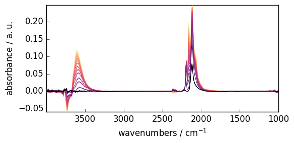
Let’s import a group of IR spectra, look at its content and plot it:
[4]:
X = scp.read_omnic("irdata/CO@Mo_Al2O3.SPG", description="CO adsorption, diff spectra")
X.y = (X.y - X[0].y).to("minute")
X
[4]:
NDDataset [CO@Mo_Al2O3] — float64, shape: (y:19, x:3112), a.u.
2026-07-26 02:35:07+00:00> Sorted by date
Data
[-3.608e-05 -0.0001981 ... 0.0003089 0.00117]
...
[0.0008357 -0.0001387 ... -0.0005221 -0.001121]
[0.0005655 -0.000116 ... -0.00057 -0.0006307]] a.u.
Dimension `x`
Dimension `y`
[ *Résultat de Soustraction:04_Mo_Al2O3_calc_0.003torr_LT_after sulf_Oct 18 15:46:42 2016 (GMT+02:00)
*Résultat de Soustraction:04_Mo_Al2O3_calc_0.004torr_LT_after sulf_Oct 18 15:51:12 2016 (GMT+02:00) ...
*Résultat de Soustraction:04_Mo_Al2O3_calc_0.905torr_LT_after sulf_Oct 18 17:58:42 2016 (GMT+02:00)
*Résultat de Soustraction:04_Mo_Al2O3_calc_1.004torr_LT_after sulf_Oct 18 18:03:41 2016 (GMT+02:00)]]
[5]:
subplot = X.plot() # assignment avoids displaying the object address (<matplotlib.axes._subplots.AxesSubplot ...>)
Slicing with indexes
Classical slicing using integers can be used. For instance, along the 1st dimension:
[6]:
print(X[:4])  # selects the first four spectra
print(X[-3:])  # selects the last three spectra
print(X[::2])  # selects one spectrum out of 2
NDDataset: [float64] a.u. (shape: (y:4, x:3112))
NDDataset: [float64] a.u. (shape: (y:3, x:3112))
NDDataset: [float64] a.u. (shape: (y:10, x:3112))
The same can be done along the second dimension, either together with the first one or independently. For instance:
[7]:
print(
    X[:, ::2]
)  # all spectra, one wavenumber out of 2 (note: X[,::2] generates an error)
print(
    X[0:3, 200:1000:2]
)  # first 3 spectra, one wavenumber out of 2, from index 200 to 1000
NDDataset: [float64] a.u. (shape: (y:19, x:1556))
NDDataset: [float64] a.u. (shape: (y:3, x:400))
Would you easily guess which wavenumber range has actually been selected? Probably not, because the relationship between the index and the wavenumber is not straightforward as it depends on the value of the first wavenumber, the wavenumber spacing, and whether the wavenumbers are arranged in ascending or descending order… Here is the answer:
[8]:
X[
    :, 200:1000:2
].x  # as the Coord can be sliced, the same is obtained with: X.x[200:1000:2]
[8]:
Coord [x:wavenumbers] — float64, size: 400, cm⁻¹
Slicing with coordinates
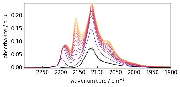
Now the spectroscopist is generally interested in a particular region of the spectrum, for instance, 2300-1900 cm\(^{-1}\). Can you easily guess the indices that should be used to select this region? Probably not without a calculator.
Fortunately, a simple mechanism has been implemented in SpectroChemPy for this purpose: the use of floats instead of integers will slice the NDDataset at the corresponding coordinates. For instance, to select the 2300-1900 cm\(^{-1}\) region:
[9]:
subplot = X[:, 2300.0:1900.0:].plot()
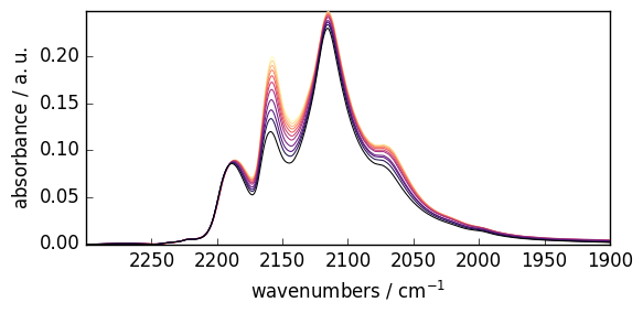
The same mechanism can be used along the first dimension (y). For instance, to select and plot the same region and the spectra recorded between 80 and 180 minutes:
[10]:
subplot = X[
    80.0:180.0, 2300.0:1900.0
].plot()  # Note that a decimal point is enough to create a float
# a warning is raised if one or several values are beyond the limits
INFO | This coordinate (180.0) is outside the axis limits (0.0-137.033).
The closest limit index is returned
Similarly, the spectrum recorded closest to 60 minutes can be selected using a float:
[11]:
X[60.0].y # X[60.] slices the spectrum; .y returns the corresponding `y` axis.
[11]:
Coord [y:acquisition timestamp (GMT)] — float64, size: 1, min
[ *Résultat de Soustraction:04_Mo_Al2O3_calc_0.021torr_LT_after sulf_Oct 18 16:45:00 2016 (GMT+02:00)]]
— End of Tutorial — (todo: add advanced slicing by array of indices, array of bool, …)