× ⚠️ You are reading the development version documentation.
Read here the documentation of the last stable release.

Introduction to the plotting library

This short gallery example shows three common ideas:

• the default dataset.plot() entry point;

• per-call style changes that do not mutate later plots;

• plot_multiple() overlaying several 1D datasets on one shared axes.

import os
from pathlib import Path

import numpy as np
import spectrochempy as scp

Locate and load a dataset

datadir = scp.preferences.datadir
TEST_FILE = Path(
    os.environ.get("TEST_FILE", datadir / "irdata" / "nh4y-activation.spg")
)
dataset = scp.read(TEST_FILE)

Default plot and style

ax = dataset[0].plot()

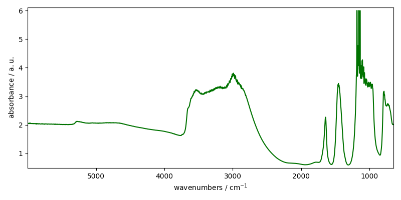
Per-call style changes

Apply a style to this single plot only:

ax = dataset[0].plot(style="classic")

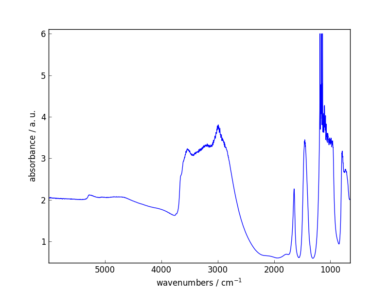
The style change is local — the default style is used again here:

ax = dataset[0].plot()

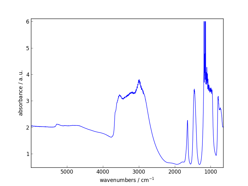
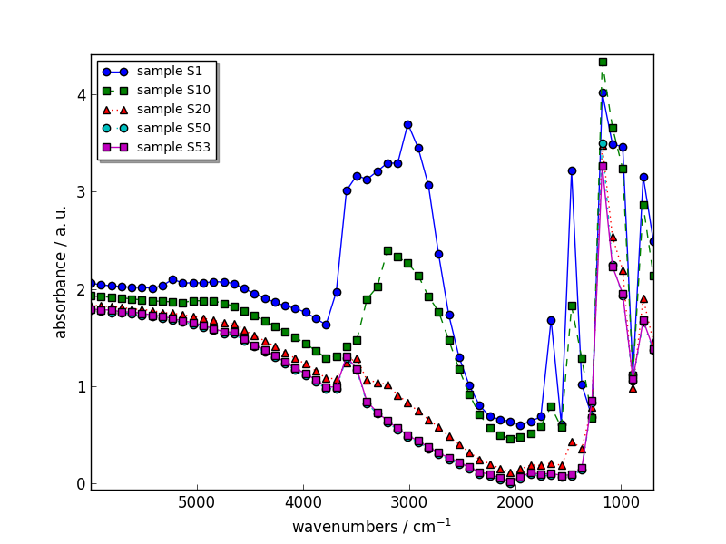
Overlay with plot_multiple

dataset = dataset[:, ::100]

sample_indices = np.linspace(0, dataset.shape[0] - 1, 5, dtype=int)
datasets = [dataset[index] for index in sample_indices]
labels = [f"sample {index}" for index in sample_indices]

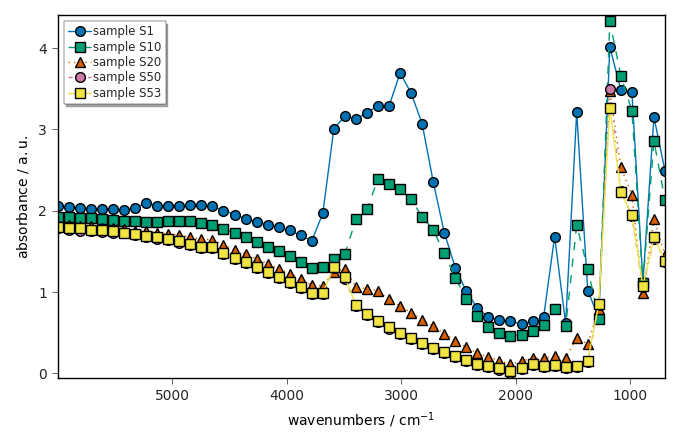
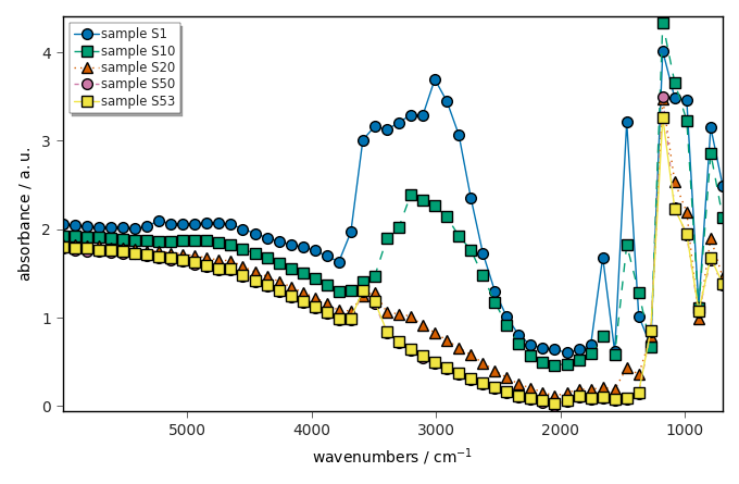
_ = scp.plot_multiple(method="scatter", datasets=datasets, labels=labels, legend="best")

The style change applies only to this call:

_ = scp.plot_multiple(
    method="scatter", style="sans", datasets=datasets, labels=labels, legend="best"
)

The default style is used again on the next call:

_ = scp.plot_multiple(method="scatter", datasets=datasets, labels=labels, legend="best")

This ends the example ! The following line can be uncommented if no plot shows when running the .py script with python

# scp.show()