spectrochempy.PLSRegression

class PLSRegression(*, log_level='WARNING', warm_start=False, max_iter=500, n_components=2, scale=True, tol=1e-06)[source]

Parameters:

max_iter (int, optional, default: 500) – The maximum number of iterations of the power method when algorithm=’nipals’. Ignored otherwise.
n_components (int, optional, default: 2) – Number of components to keep. Should be in the range [1, min(n_samples, n_features, n_targets)].
scale (bool, optional, default: True) – Whether to scale X and Y.
tol (float, optional, default: 1e-06) – The tolerance used as convergence criteria in the power method:the algorithm stops whenever the squared norm of u_i - u_{i-1} is less than tol, where u corresponds to the left singular vector.

Initialize the BaseConfigurable class.

Parameters:

log_level (int, optional) – The log level at startup. Default is logging.WARNING.
**kwargs (dict) – Additional keyword arguments for configuration.

Attributes Summary

`X`	Return the X input dataset (eventually modified by the model).
`Y`	The `Y` input.
`components`	`NDDataset` with components in feature space (n_components, n_features).
`config`	`traitlets.config.Config` object.
`log`	Return `log` output.
`max_iter`	The maximum number of iterations of the power method when algorithm='nipals'.
`n_components`	Number of components to keep.
`name`	Object name
`scale`	Whether to scale X and Y.
`tol`	the algorithm stops whenever the squared norm of u_i - u_{i-1} is less than tol, where u corresponds to the left singular vector.

Methods Summary

`fit`(X, Y)	Fit the PLSRegression model on X and Y.
`fit_transform`(X, Y[, both])	Fit the model with `X` and `Y` and apply the dimensionality reduction on `X` and optionally on `Y`.
`get_components`([n_components])	Return the component's dataset: (selected n_components, n_features).
`get_params`([deep])	Get the configuration parameters of this estimator.
`inverse_transform`([X_transform, ...])	Transform data back to its original space.
`params`([default])	Return current or default configuration values.
`parityplot`([replace, removed, Y, Y_hat, ax, ...])	Backward-compatible alias for `plot_parity`.
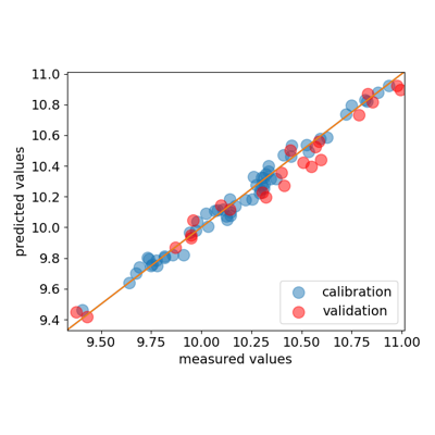
`plot_merit`([X, X_hat])	Plot the input (`X`), reconstructed (`X_hat`) and residuals.
`plot_parity`(self[, Y, Y_hat, ax, clear, show])	Plot the predicted (\(\hat{Y}\)) vs measured (\(Y\)) values.
`plotmerit`([replace, removed, X, X_hat])	Backward-compatible alias for `plot_merit`.
`predict`([X])	Predict targets of given observations.
`reset`()	Reset configuration parameters to their default values.
`score`([X, Y, sample_weight])	Return the coefficient of determination of the prediction.
`set_params`(**params)	Set configuration parameters on this estimator.
`to_dict`()	Return config value in a dict form.
`transform`([X, Y, both])	Apply dimensionality reduction to X`and `Y.

Attributes Documentation

X: Return the X input dataset (eventually modified by the model).

Y: The Y input.

components

NDDataset with components in feature space (n_components, n_features).

See also

get_components: Retrieve only the specified number of components.

config: traitlets.config.Config object.

log: Return log output.

max_iter: The maximum number of iterations of the power method when algorithm=’nipals’. Ignored otherwise.

n_components: Number of components to keep. Should be in the range [1, min(n_samples, n_features, n_targets)].

name: Object name

scale: Whether to scale X and Y.

tol

the algorithm stops whenever the squared norm of u_i - u_{i-1} is less than tol, where u corresponds to the left singular vector.

Type:: The tolerance used as convergence criteria in the power method

Methods Documentation

fit(X, Y)[source]

Fit the PLSRegression model on X and Y.

Parameters:

X (NDDataset or array-like of shape (n_observations, n_features)) – Training data.
Y (array-like of shape (n_samples,) or (n_samples, n_targets)) – Target vectors, where n_samples is the number of samples and n_targets is the number of response variables.

Returns:

self – The fitted instance itself.

See also

fit_transform: Fit the model with an input dataset X and apply the dimensionality reduction on X.

fit_transform(X, Y, both=False)[source]

Fit the model with X and Y and apply the dimensionality reduction on X and optionally on Y.

Parameters:

X (NDDataset or array-like of shape (n_observations, n_features)) – Training data.
Y (NDDataset or array-like of shape (n_observations, n_features)) – Training data.
both (bool, optional) – Whether to also apply the dimensionality reduction to Y when neither X nor Y are provided.

Returns:

NDDataset or tuple of NDDataset – Transformed data.

get_components(n_components=None)

Return the component’s dataset: (selected n_components, n_features).

Parameters:: n_components (int, optional, default: None) – The number of components to keep in the output dataset. If None, all calculated components are returned.
Returns:: NDDataset – Dataset with shape (n_components, n_features)

get_params(deep=True)[source]

Get the configuration parameters of this estimator.

Parameters:: deep (bool, optional, default:True) – Ignored. Present for compatibility with scikit-learn conventions.
Returns:: dict – Mapping of parameter name -> current value.

inverse_transform(X_transform=None, Y_transform=None, both=False, **kwargs)

Transform data back to its original space.

In other words, return reconstructed X and Y whose reduce/transform would be X_transform and Y_transform.

Parameters:

X_transform (array-like of shape (n_observations, n_components), optional) – Reduced X data, where n_observations is the number of observations and n_components is the number of components. If X_transform is not provided, a transform of X provided in fit is performed first.
Y_transform (NDDataset or array-like of shape (n_observations, n_components), optional) – New data, where n_targets is the number of variables to predict. If Y_transform is not provided, a transform of Y provided in fit is performed first.
**kwargs (keyword parameters, optional) – See Other Parameters.

Returns:

NDDataset – Dataset with shape (n_observations, n_components).

Other Parameters:

n_components (int, optional) – The number of components to use for the reduction.

See also

reconstruct: Alias of inverse_transform (Deprecated).

params(default=False)[source]

Return current or default configuration values.

Parameters:: default (bool, optional, default: False) – If default is True, the default parameters are returned, else the current values.
Returns:: dict – Current or default configuration values.

parityplot(replace="plot_parity", removed="0.12") def parityplot( self, Y=None, Y_hat=None, *, ax=None, clear=True, show=True, **kwargs)[source]

Backward-compatible alias for plot_parity. Deprecated.

Returns:: Axes – Matplotlib axes containing the parity plot.

plot_merit(X=None, X_hat=None, **kwargs)[source]

Plot the input (X), reconstructed (X_hat) and residuals.

\(X\) and \(\hat{X}\) can be passed as arguments. If not, the X attribute is used for \(X`and :math:\)hat{X}`is computed by the inverse_transform method

Parameters:

X (NDDataset, optional) – Original dataset. If is not provided (default), the X attribute is used and X_hat is computed using inverse_transform.
X_hat (NDDataset, optional) – Inverse transformed dataset. if X is provided, X_hat must also be provided as compuyed externally.

Returns:

Axes – Matplotlib subplot axe.

Other Parameters:

exp_c (color, colormap, or list of colors, optional) – Color(s) for experimental spectra. - None: use unified semantic resolver (auto-detect categorical/sequential) - Single color: use for all experimental spectra - Colormap name/object: sample colors from colormap - List/tuple: use as explicit color cycle
calc_c (color, colormap, or list of colors, optional) – Color(s) for calculated spectra. - None: use default blue “#2a6fbb” - Single color: use for all calculated spectra - Colormap name/object: sample colors from colormap - List/tuple: use as explicit color cycle
resid_c (color, colormap, or list of colors, optional) – Color(s) for residual spectra. - None: use default grey “0.4” - Single color: use for all residual spectra - Colormap name/object: sample colors from colormap - List/tuple: use as explicit color cycle
exp_linestyle (str, optional) – Line style for experimental spectra. Default: “-“.
calc_linestyle (str, optional) – Line style for calculated spectra. Default: “–“.
resid_linestyle (str, optional) – Line style for residual spectra. Default: “-“.
exp_linewidth (float, optional) – Line width for experimental spectra. Default: 1.2.
calc_linewidth (float, optional) – Line width for calculated spectra. Default: 1.0.
resid_linewidth (float, optional) – Line width for residual spectra. Default: 1.0.
min_contrast (float, optional) – Minimum contrast ratio for sequential colormaps. Default: 1.5.
offset (float, optional, default: None) – Specify the separation (in percent) between the \(X\) , \(X_hat\) and \(E\).
nb_traces (int or 'all', optional) – Number of lines to display. Default is 'all'.
**others (Other keywords parameters) – Parameters passed to the internal plot method of the X dataset. Common options include color, linewidth, linestyle, alpha, and standard Matplotlib kwargs.

plot_parity(self, Y=None, Y_hat=None, *, ax=None, clear=True, show=True, **kwargs)[source]

Plot the predicted (\(\hat{Y}\)) vs measured (\(Y\)) values.

\(Y\) and \(\hat{Y}\) can be passed as arguments. If not, the Y attribute is used for \(\hat{Y}\) computed by the predict method.

Parameters:

Y (NDDataset, optional) – Measured values. If not provided, uses self.Y and computes Y_hat via self.predict(self.X).
Y_hat (NDDataset, optional) – Predicted values. If Y is provided, Y_hat must also be provided as computed externally.
ax (Axes, optional) – Axes to plot on. If None, a new figure is created.
clear (bool, optional) – Whether to clear the axes before plotting. Default: True. Only used when ax is provided.
show (bool, optional) – Whether to display the figure. Default: True.
**kwargs (keyword arguments, optional) – Additional keyword arguments passed to scatter. Includes s, c, marker, cmap, norm, vmin, vmax, alpha, linewidths, edgecolors, plotnonfinite.

Returns:

Axes – Matplotlib axes containing the parity plot.

See also

parityplot: Deprecated alias for this method.

plotmerit(replace="plot_merit", removed="0.12") def plotmerit(self, X=None, X_hat=None, **kwargs)[source]

Backward-compatible alias for plot_merit. Deprecated.

Returns:: Axes – Matplotlib axes containing the plot.

predict(X=None)

Predict targets of given observations.

Parameters:: X (NDDataset or array-like of shape (n_observations, n_features), optional) – New data, where n_observations is the number of observations and n_features is the number of features. if not provided, the input dataset of the fit method will be used.
Returns:: NDDataset – Datasets with shape (n_observations,) or ( n_observations, n_targets).

reset()[source]: Reset configuration parameters to their default values.

score(X=None, Y=None, sample_weight=None)[source]

Return the coefficient of determination of the prediction.

The coefficient of determination \(R^2\) is defined as \((1 - \frac{u}{v})\) , where \(u\) is the residual sum of squares ((y_true - y_pred)** 2).sum() and \(v\) is the total sum of squares ((y_true - y_true.mean()) ** 2).sum(). The best possible score is 1.0 and it can be negative (because the model can be arbitrarily worse). A constant model that always predicts the expected value of Y, disregarding the input features, would get a \(R^2\) score of 0.0.

Parameters:

X (NDDataset or array-like of shape (n_observations, n_features), optional) – Test samples. If not given, the X attribute is used.
Y (NDDataset or array-like of shape (n_observations, n_targets), optional) – True values for X.
sample_weight (NDDataset or array-like of shape (n_samples,), default: None) – Sample weights.

Returns:

float – \(R^2\) of predict`(X) w.r.t `Y.

set_params(**params)[source]

Set configuration parameters on this estimator.

Returns self so that calls can be chained.

Parameters:: **params – Parameter names and values to update.
Returns:: self – The estimator instance.
Raises:: SpectroChemPyError – If a parameter name does not correspond to a configurable trait.

to_dict()[source]

Return config value in a dict form.

Returns:: dict – A regular dictionary.

transform(X=None, Y=None, both=False, **kwargs)

Apply dimensionality reduction to X`and `Y.

Parameters:

X (NDDataset or array-like of shape (n_observations, n_features), optional) – New data, where n_observations is the number of observations and n_features is the number of features. if not provided, the input dataset of the fit method will be used.
Y (NDDataset or array-like of shape (n_observations, n_targets), optional) – New data, where n_targets is the number of variables to predict. if not provided, the input dataset of the fit method will be used.
both (bool, default: False) – Whether to also apply the dimensionality reduction to Y when neither X nor Y are provided.

Returns:

x_score, y_score (NDDataset or tuple of NDDataset) – Datasets with shape (n_observations, n_components).

Examples using spectrochempy.PLSRegression

PLS regression example