SIMPLISMA example

In this example, we perform the PCA dimensionality reduction of a spectra dataset

Import the package

import spectrochempy as scp

Load and annotate the dataset

print("Dataset (Jaumot et al., Chemometr. Intell. Lab. 76 (2005) 101-110)):")
lnd = scp.read_matlab("matlabdata/als2004dataset.MAT", merge=False)
for mat in lnd:
    print("    " + mat.name, str(mat.shape))

ds = lnd[-1]
_ = ds.plot()

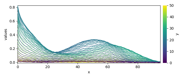
Dataset (Jaumot et al., Chemometr. Intell. Lab. 76 (2005) 101-110)):
    cpure (204, 4)
    MATRIX (204, 96)
    isp_matrix (4, 4)
    spure (4, 96)
    csel_matrix (51, 4)
    m1 (51, 96)

Add metadata for a nicer display:

ds.title = "absorbance"
ds.units = "absorbance"
ds.set_coordset(None, None)
ds.y.title = "elution time"
ds.x.title = "wavelength"
ds.y.units = "hours"
ds.x.units = "nm"

Fit the SIMPLISMA model

print("Fit SIMPLISMA on {}\n".format(ds.name))
simpl = scp.SIMPLISMA(n_components=20, tol=0.2, noise=3, log_level="INFO")
_ = simpl.fit(ds)

Fit SIMPLISMA on m1

/home/runner/work/spectrochempy/spectrochempy/.venv/lib/python3.13/site-packages/traitlets/traitlets.py:1576: UserWarning: SIMPLISMA does not handle easily negative values.
  c(event)
 *** Automatic SIMPL(I)SMA analysis ***
      dataset: m1
        noise: 3.0 %
          tol: 0.2 %
 n_components: 20


 #iter index_pc  coord_pc   Std(res)   R^2
 ---------------------------------------------
    1      4       4.0     0.0263     0.9755
    2     82      82.0     0.0100     0.9964
    3     29      29.0     0.0072     0.9981
 **** Unexplained variance lower than 'tol' (0.2 %)
 **** End of SIMPL(I)SMA analysis.

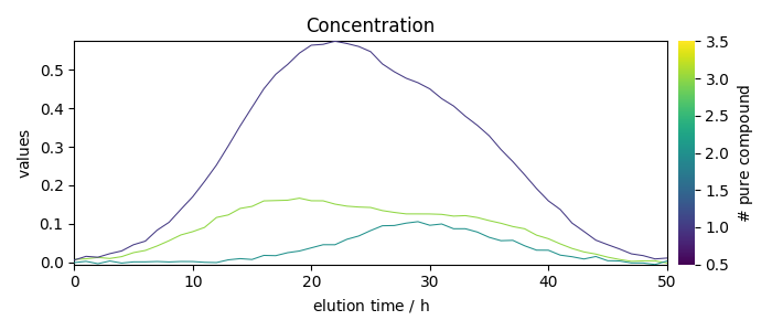
Visualize the results

Concentration profiles:

_ = simpl.C.T.plot(title="Concentration")

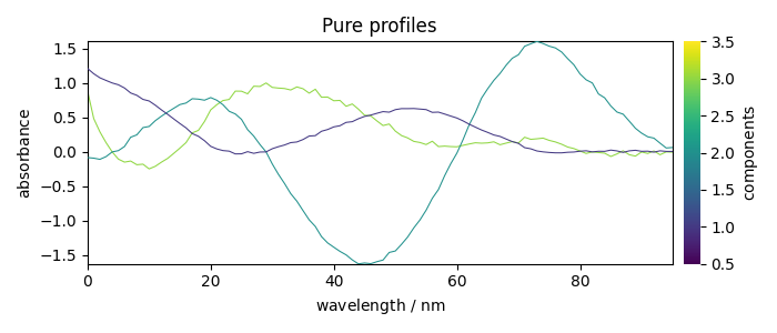
Pure component spectra:

_ = simpl.components.plot(title="Pure profiles")

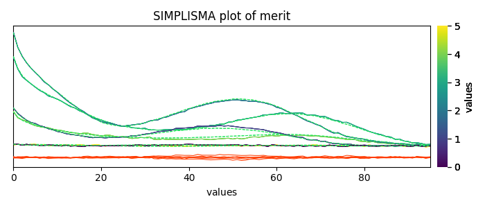
Merit plot after reconstruction:

_ = simpl.plot_merit(offset=0, nb_traces=5)

This ends the example ! The following line can be uncommented if no plot shows when running the .py script with python

# scp.show()

Total running time of the script: (0 minutes 0.708 seconds)