× ⚠️ You are reading the development version documentation.
Read here the documentation of the last stable release.

Fitting

import numpy as np

import spectrochempy as scp
from spectrochempy import ur

Solving a linear equation using the least square method (LSTSQ)

In the first example, we find the least square solution of a simple linear equation.

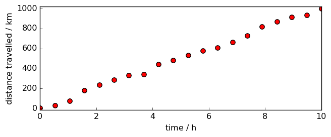
Let’s first create a NDDataset with some data. We have for instance some noisy data that represent the distance d traveled by some objects versus time t:

def func(t, v, var):
    d = v * t + (np.random.rand(len(t)) - 0.5) * var
    d[0].data = 0.0
    return d


time = scp.Coord.linspace(0, 10, 20, title="time", units="hour")
d = scp.fromfunction(
    func,
    v=100.0 * ur("km/hr"),
    var=60.0 * ur("km"),
    # extra arguments passed to the function v, var
    coordset=scp.CoordSet(t=time),
    name="mydataset",
    title="distance travelled",
)

Here is a plot of these data-points:

prefs = scp.preferences
prefs.figure.figsize = (7, 3)
_ = d.plot_scatter(markersize=7, mfc="red", label="Original data")

We want to fit a line through these data-points of equation

\(d = v.t + d_0\)

By construction, we know already that the line should have a gradient of roughly 100 km/h and cut the y-axis at, more or less, 0 km.

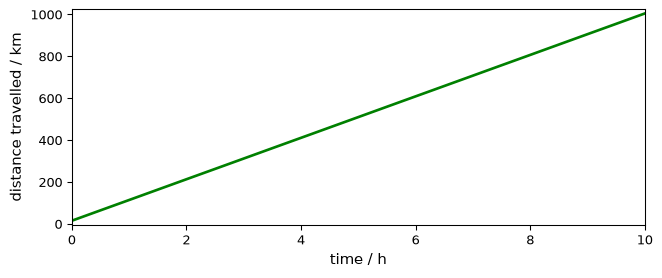
Using LSTSQ, the solution is found very easily:

lst = scp.LSTSQ()
_ = lst.fit(time, d)

v, d0 = lst.coef, lst.intercept
print(f"speed : {v:.3f},  distance at time 0 : {d0:.3f}")

dfit = lst.predict()
_ = dfit.plot_pen(clear=False, color="g", lw=2, label=" Fitted line", legend="best")

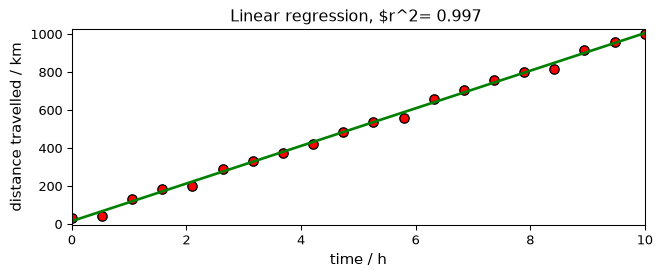
speed : 98.940 kilometer hour^-1,  distance at time 0 : 14.427 kilometer

Note

In the particular case where the variation is proportional to the x dataset coordinate, the same result can be obtained directly using d as a single parameter on LSTSQ (as t is the x coordinate axis!)

lst = scp.LSTSQ()
_ = lst.fit(d)
v, d0 = lst.coef, lst.intercept

and the final plot

_ = d.plot_scatter(
    markersize=7,
    mfc="red",
    mec="black",
    label="Original data",
    title=f"Linear regression, $r^2={lst.score(): .3f} ",
)
dfit = lst.predict()
_ = dfit.plot_pen(clear=False, color="g", lw=2, label=" Fitted line", legend="best")

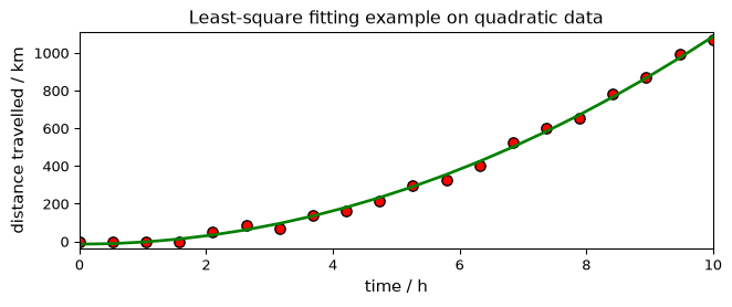
Let’s try now with a quadratic increase of the speed:

def func(t, a, var):
    d = a * (t / 3.0) ** 2 + (np.random.rand(len(t)) - 0.8) * var
    for i in range(t.size):
        if d[i].magnitude < 0:
            d[i] = 0.0 * d.units
    return d


time = scp.Coord.linspace(0, 10, 20, title="time", units="hour")
d2 = scp.NDDataset.fromfunction(
    func,
    a=100.0 * ur("km/hr^2"),
    var=60.0 * ur("km"),
    # extra arguments passed to the function v, var
    coordset=scp.CoordSet(t=time),
    name="mydataset",
    title="distance travelled",
)

_ = d2.plot_scatter(markersize=7, mfc="red")

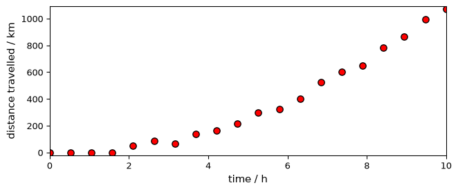
Now we must use the first syntax LSTQ(X, Y) as the variation is not proportional to time, but to its square.

X = time**2
lst = scp.LSTSQ()
_ = lst.fit(X, d2)

v, d0 = lst.coef, lst.intercept
print(f"acceleration : {v:.3f},  distance at time 0 : {d0:.3f}")

acceleration : 11.007 kilometer hour^-2,  distance at time 0 : -15.244 kilometer

_ = d2.plot_scatter(
    markersize=7,
    mfc="red",
    mec="black",
    label="Original data",
    title="Least-square fitting example on quadratic data",
)
dfit = lst.predict()

_ = dfit.plot_pen(clear=False, color="g", lw=2, label=" Fitted line", legend="best")

Least square with non-negativity constraint (NNLS)

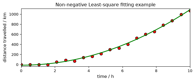
When fitting data with LSTSQ, it happens that we get some negative values were it should not, for instance having a negative distance at time 0.

In this case, we can use the NNLS method of fitting. It operates as LSTSQ but keep the Y values always positive.

X = time**2
nls = scp.NNLS()
_ = nls.fit(X, d2)

v, d0 = lst.coef, lst.intercept
print(f"acceleration : {v: .3f},  distance at time 0 : {d0: .3f}")

acceleration :  11.007 kilometer hour^-2,  distance at time 0 : -15.244 kilometer

_ = d2.plot_scatter(
    markersize=7,
    mfc="red",
    mec="black",
    label="Original data",
    title="Non-negative Least-square fitting example",
)
dfit = lst.predict()

_ = dfit.plot_pen(clear=False, color="g", lw=2, label=" Fitted line", legend="best")

NDDataset modelling using non-linear optimisation method

First we will load an IR dataset

nd = scp.read("irdata/nh4y-activation.spg")

As we want to start with a single 1D spectra, we select the last one (index -1)

nd = nd[-1].squeeze()
# nd[-1] returns a nddataset with shape (1,5549)
# this is why we squeeze it to get a pure 1D dataset with shape (5549,)

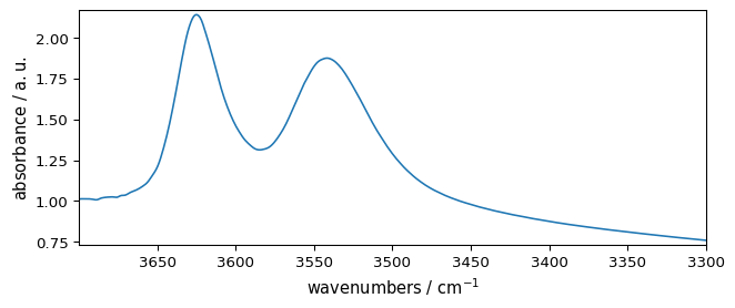
Now we slice it to keep only the OH vibration region:

ndOH = nd[3700.0:3300.0]
_ = ndOH.plot()

Baseline correction

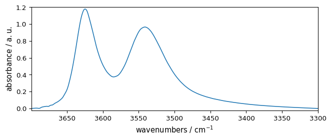
We can perform a linear baseline correction to start with this data (see the :doc:baseline tutorial </userguide/processing/baseline>). For removing a linear baseline, the fastest method is however to use the abc ( automatic baseline correction)

ndOHcorr = scp.basc(ndOH)
_ = ndOHcorr.plot()

Peak finding

Below we will need to start with some guess of the peak position and width. For this we can use the find_peaks() method (see :doc:Peak finding tutorial </userguide/analysis/peak_finding>)

peaks, _ = ndOHcorr.find_peaks()
peaks.x.values

Magnitude	[3693.693 3678.355 3624.857 3541.323]
Units	cm-1

ax = ndOHcorr.plot_pen()  # output the spectrum on ax. ax will receive next plot too
pks = peaks + 0.01  # add a small offset on the y position of the markers
_ = pks.plot_scatter(
    ax=ax,
    marker="v",
    color="black",
    clear=False,  # we need to keep the previous output on ax
    data_only=True,  # we don't need to redraw all things like labels, etc...
    ylim=(-0.05, 1.3),
)

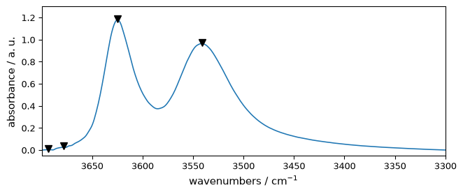
The maximum of the two major peaks are thus exactly at 3624.61 and 3541.68 cm\(^{-1}\)

Fitting script

Now we will define the fitting procedure as a script

script = """

#-----------------------------------------------------------
# syntax for parameters definition :
# name : value, low_bound,  high_bound
#  * for fixed parameters
#  $ for variable parameters
#  > for reference to a parameter in the COMMON block
#    (> is forbidden in the COMMON block)
# common block parameters should not have a _ in their names
#-----------------------------------------------------------
#
COMMON:
# common parameters ex.
# $ gwidth: 1.0, 0.0, none
$ gratio: 0.1, 0.0, 1.0
$ gasym: 0.1, 0, 1

MODEL: LINE_1
shape: asymmetricvoigtmodel
    * ampl:  1.0, 0.0, none
    $ pos:   3624.61, 3610.0, 3640.0
    > ratio: gratio
    > asym: gasym
    $ width: 200, 0, 1000

MODEL: LINE_2
shape: asymmetricvoigtmodel
    $ ampl:  0.2, 0.0, none
    $ pos:   3541.68, 3520.0, 3560.0
    > ratio: gratio
    > asym: gasym
    $ width: 200, 0, 1000

"""

Syntax for parameters definition

In such script, the char # at the beginning of a line denote that the whole line is a comment. Comments are obviously optional but may be useful to explain

Each individual model component is identified by the keyword MODEL

A MODEL have a name, e.g., MODEL: LINE_1 .

Then come for each model components its shape , i.e., the shape of the line.

Come after the definition of the model parameters depending on the shape, e.g., for a gaussianmodel we have three parameters: amplitude (ampl), width and position (pos) of the line.

To define a given parameter, we have to write its name and a set of 3 values: the expected value and 2 limits for the allowed variations : low_bound, high_bound:

name : value, low_bound,  high_bound

These parameters are preceded by a mark saying what kind of parameter it will behave in the fit procedure:

• $ is the default and denote a variable parameters

• * denotes fixed parameters

• > say that the given parameters is actually defined in a COMMON block

COMMONis the common block containing parameters to which a parameter in the MODEL blocks can make reference using the > markers. (> obviously is forbidden in the COMMON block) common block parameters should not have a _(underscore) in their names

With this parameter script definition, you can thus make rather complex search for modelling, as you can make parameters dependents or fixed.

The line shape can be (up to now) in the following list of shape (for 1D models - see below for 2D):

• PolynomialBaseline -> polynomialbaseline:

  Arbitrary-degree polynomial (degree limited to 10, however). As a linear baseline is automatically calculated during fitting, this polynom is always of greater or equal to order 2 (parabolic function at the minimum).

  \(f(x) = ampl * \sum_{i=2}^{max} c_i*x^i\)

  MODEL: baseline
  shape: polynomialbaseline
  # This polynomial starts at the order 2
  $ ampl: val, 0.0, None
  $ c_2: 1.0, None, None
  * c_3: 0.0, None, None
  * c_4: 0.0, None, None
  # etc
  

• Gaussian Model -> gaussianmodel:

  Normalized 1D gaussian function.

  \(f(x) = \frac{ampl}{\sqrt{2 \pi \sigma^2}} \exp({\frac{-(x-pos)^2}{2 \sigma^2}})\)

  where \(\sigma = \frac{width}{2.3548}\)

  MODEL: Linex
  shape: gaussianmodel
  $ ampl: val, 0.0, None
  $ width: val, 0.0, None
  $ pos: val, lob,  upb
  

• Lorentzian Model -> lorentzianmodel:

  A standard Lorentzian function (also known as the Cauchy distribution).

  \(f(x) = \frac{ampl * \lambda}{\pi [(x-pos)^2+ \lambda^2]}\)

  where \(\lambda = \frac{width}{2}\)

  MODEL: liney:
  shape: lorentzianmodel
  $ ampl:val, 0.0, None
  $ width: val, 0.0, None
  $ pos: val, lob, upb
  

• Voigt Model -> voigtmodel:

  A Voigt model constructed as the convolution of a GaussianModel and a LorentzianModel – commonly used for spectral line fitting.

  MODEL: linez
  shape: voigtmodel
  $ ampl: val, 0.0, None
  $ width: val, 0.0, None
  $ pos: val, lob, upb
  $ ratio: val, 0.0, 1.0
  

• Asymmetric Voigt Model -> asymmetricvoigtmodel:

  An asymmetric Voigt model (A. L. Stancik and E. B. Brauns, Vibrational Spectroscopy, 2008, 47, 66-69)

  MODEL: linez
  shape: voigtmodel
  $ ampl: val, 0.0, None
  $ width: val, 0.0, None
  $ pos: val, lob, upb
  $ ratio: val, 0.0, 1.0
  $ asym: val, 0.0, 1.0
  

For quick synthetic profiles outside the fitting workflow, SpectroChemPy also exposes direct helpers at the top level: scp.gaussian, scp.lorentzian, scp.voigt, scp.asymmetricvoigt, and scp.sigmoid.

Validate the script before fitting

You do not have to wait for the fit to discover errors in the script. Call :meth:~spectrochempy.analysis.curvefitting.optimize.Optimize.validate_script to check the script before launching the optimisation:

f1 = scp.Optimize(log_level="INFO")
errors = f1.validate_script(script)
errors  # should be an empty list if the script is valid

[]

If the script contains an error, errors will contain :class:~spectrochempy.analysis.curvefitting.optimize.ScriptError objects with the line number, the offending line, and a human-readable explanation. An empty list means the script is syntactically correct and all model references are recognised.

Optimize also exposes validate_constraints() for lightweight validation of constraint specifications before fitting. At the moment this is deliberately a narrow surface: it validates the structure of recognized constraint specs and any referenced parameter names from the script, but it should not yet be read as a complete guarantee of backend-level constraint enforcement.

The currently supported minimal schema is intentionally small. For example, the following constraint specification is accepted and normalized:

constraint_spec = {"max_connections": 2}
f1.validate_constraints(constraint_spec)
f1.constraints = constraint_spec
f1.constraints

{'type': 'max_connections', 'limit': 2, 'parameters': None}

This currently demonstrates validation and normalization of the public constraint surface. It should not yet be read as a promise of rich constraint semantics during optimization. The short form shown above is normalized to the canonical stored form:

• short form: {"max_connections": 2}

• canonical form: {"type": "max_connections", "limit": 2, "parameters": None}

Choosing a fitting method

Optimize currently exposes four public values for method:

• least_squares

• leastsq

• simplex

• basinhopping

In practice, these fall into three maintained families:

Public method	Current role	Type of search	Current internal path	Jacobian / covariance path
least_squares	recommended local least-squares entrypoint	local least-squares fit	SciPy least_squares()	yes, when available
leastsq	compatibility alias	local least-squares fit	same SciPy least_squares() path	yes, when available
simplex	derivative-free local fallback	local derivative-free search	SciPy simplex (fmin) path	no
basinhopping	exploratory global-style option	global-style exploratory search	SciPy basinhopping()	no

The main user-facing guidance is:

• start with least_squares for ordinary peak fitting and most well-initialized models;

• treat leastsq mainly as a backwards-compatible spelling, not as a distinct maintained strategy;

• try simplex when you want a derivative-free local search and can accept losing the least-squares uncertainty path;

• try basinhopping only when the landscape is difficult enough to justify a slower exploratory search.

The current implementation automatically chooses between the least-squares backend variants lm and trf depending on the size of the varying-parameter problem. This choice is internal: users select the high-level method, not the low-level SciPy backend directly.

method_summary = {
    "recommended_default": "least_squares",
    "compatibility_alias": "leastsq",
    "derivative_free_local": "simplex",
    "exploratory_global": "basinhopping",
}
method_summary

{'recommended_default': 'least_squares',
 'compatibility_alias': 'leastsq',
 'derivative_free_local': 'simplex',
 'exploratory_global': 'basinhopping'}

Other useful fitting modes

Several public options affect how a fit is prepared:

• dry=True validates the script and assembles the starting model without running the optimizer;

• autobase=True adds an automatic baseline correction step before fitting;

• autoampl=True adjusts initial amplitudes automatically;

• amplitude_mode="height" or "area" controls how line-shape amplitudes are initialized;

• warm_start=True preserves the current estimator configuration instead of forcing a full reset to default configuration values during estimator reinitialization.

These options do not all answer the same question:

• method chooses how the numerical search is run;

• dry, autobase, autoampl, and amplitude_mode help define how the fit starts;

• warm_start is a broader estimator-state option and should not be read as a dedicated Optimize solver warm-start backend.

The availability of advanced post-fit quantities depends on the chosen method. Least-squares-backed methods can expose a retained Jacobian and therefore the uncertainty path (covariance, stderr, correlation, confidence_intervals). simplex and basinhopping still produce fitted curves and residual diagnostics, but they do not currently expose the same uncertainty information.

f1.script = script
f1.max_iter = 2000
# f1.autobase = True
_ = f1.fit(ndOHcorr)

 **************************************************
 Result:
 **************************************************

 COMMON:
        $ gratio:     0.5474, 0.0, 1.0
        $ gasym:     0.8842, 0.0, 1.0

 MODEL: line_1
 shape: asymmetricvoigtmodel
        * ampl:     1.0000, 0.0, none
        > asym:gasym
        $ pos:  3622.7494, 3610.0, 3640.0
        > ratio:gratio
        $ width:    48.6369, 0.0, 1000.0

 MODEL: line_2
 shape: asymmetricvoigtmodel
        $ ampl:     0.9059, 0.0, none
        > asym:gasym
        $ pos:  3537.1347, 3520.0, 3560.0
        > ratio:gratio
        $ width:    77.5669, 0.0, 1000.0

fitted = f1.result.fitted
components = f1.result.components

f1.result groups fitted outputs and diagnostics without removing the existing direct estimator surface. Direct access such as f1.components, f1.predict(), and plotting helpers remains supported.

f1.result.parameters stores the configuration snapshot of the completed run: method choice, iteration limits, and fit-preparation options such as dry, autobase, autoampl, amplitude_mode, and normalized constraints. It should be read as run configuration, not as a table of solved scientific parameter values.

{
    key: f1.result.parameters[key]
    for key in (
        "method",
        "max_iter",
        "dry",
        "autobase",
        "autoampl",
        "amplitude_mode",
        "constraints",
    )
}

{'method': 'least_squares',
 'max_iter': 2000,
 'dry': False,
 'autobase': False,
 'autoampl': False,
 'amplitude_mode': 'height',
 'constraints': {'type': 'max_connections', 'limit': 2, 'parameters': None}}

Raw solver artifacts stay on the estimator. Least-squares-backed methods keep the retained Jacobian on f1.jacobian, while simplex, basinhopping, and dry fits return None. f1.result.covariance is the first scientific interpretation built on top of that Jacobian: it is an approximate local least-squares covariance matrix, scaled by the residual variance and degrees of freedom. f1.result.variance and f1.result.stderr expose the diagonal terms and standard errors derived from that covariance, and f1.result.correlation exposes the normalized parameter-correlation matrix. f1.result.confidence_intervals now exposes approximate two-sided 95% confidence intervals derived from the fitted values, standard errors, and a Student-t critical value based on the residual degrees of freedom. These quantities are only available when a backend provides a stable Jacobian and should not be confused with a full uncertainty report. Model-comparison diagnostics are also available in f1.result.diagnostics, including aic and bic.

The fitted components remain regular datasets, so they can be plotted directly against the corrected spectrum.

_ = ndOHcorr.plot()
ax = (components[:]).plot(clear=False)
ax.autoscale(enable=True, axis="y")

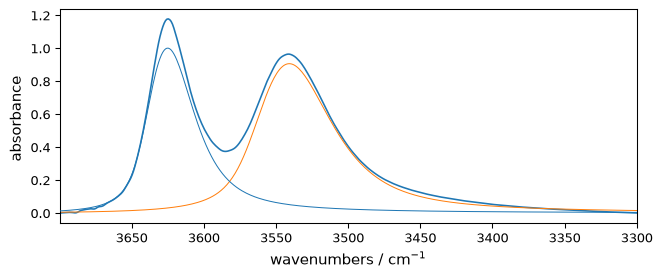
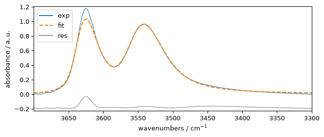
plot_merit() overlays the experimental spectrum, the fitted profile, and the residuals. Here we use a small residual offset to keep the three traces easy to inspect in a notebook. Short legend labels and an explicit legend position keep the annotation clear on the compact tutorial figure.

som = fitted
_ = f1.plot_merit(
    offset=15,
    exp_label="exp",
    calc_label="fit",
    resid_label="res",
    legend_loc="upper left",
)

Todo

Tutorial to be continued with other methods of optimization and fitting (2D…)