× ⚠️ You are reading the development version documentation.
Read here the documentation of the last stable release.

2D-IRIS analysis example

In this example, we perform the 2D IRIS analysis of CO adsorption on a sulfide catalyst.

import spectrochempy as scp

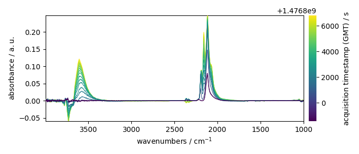
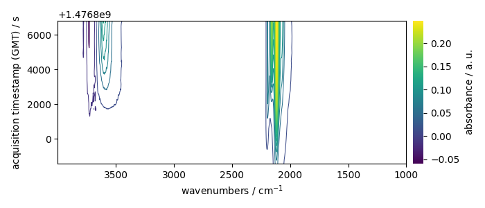
Uploading dataset

X = scp.read("irdata/CO@Mo_Al2O3.SPG")

X has two coordinates: * wavenumbers named “x” * and timestamps (i.e., the time of recording) named “y”.

print(X.coordset)

CoordSet: [x:wavenumbers, y:acquisition timestamp (GMT)]

Setting new coordinates

The y coordinates of the dataset is the acquisition timestamp. However, each spectrum has been recorded with a given pressure of CO in the infrared cell.

Hence, it would be interesting to add pressure coordinates to the y dimension:

pressures = [
    0.003,
    0.004,
    0.009,
    0.014,
    0.021,
    0.026,
    0.036,
    0.051,
    0.093,
    0.150,
    0.203,
    0.300,
    0.404,
    0.503,
    0.602,
    0.702,
    0.801,
    0.905,
    1.004,
]

c_pressures = scp.Coord(pressures, title="pressure", units="torr")

Now we can set multiple coordinates:

c_times = X.y.copy()  # the original coordinate
X.y = [c_times, c_pressures]
print(X.y)

CoordSet: [_1:acquisition timestamp (GMT), _2:pressure]

To get a detailed a rich display of these coordinates. In a jupyter notebook, just type:

X.coordset

CoordSet: [x:wavenumbers, y:[_1:acquisition timestamp (GMT), _2:pressure]][CoordSet_0a4ec2b2]

Dimension `x`

size

:

3112

title

:

wavenumbers

coordinates

:

[ 4000 3999 ... 1001 999.9] cm⁻¹

Dimension `y`

size

:

19

(_1)

title

:

acquisition timestamp (GMT)

coordinates

:

[1.477e+09 1.477e+09 ... 1.477e+09 1.477e+09] s

labels

:

...

[[ 2016-10-18 13:49:35+00:00 2016-10-18 13:54:06+00:00 ... 2016-10-18 16:01:33+00:00 2016-10-18 16:06:37+00:00]
[ *Résultat de Soustraction:04_Mo_Al2O3_calc_0.003torr_LT_after sulf_Oct 18 15:46:42 2016 (GMT+02:00)
*Résultat de Soustraction:04_Mo_Al2O3_calc_0.004torr_LT_after sulf_Oct 18 15:51:12 2016 (GMT+02:00) ...
*Résultat de Soustraction:04_Mo_Al2O3_calc_0.905torr_LT_after sulf_Oct 18 17:58:42 2016 (GMT+02:00)
*Résultat de Soustraction:04_Mo_Al2O3_calc_1.004torr_LT_after sulf_Oct 18 18:03:41 2016 (GMT+02:00)]]

(_2)

title

:

pressure

coordinates

:

[ 0.003 0.004 ... 0.905 1.004] torr

By default, the current coordinate is the first one (here c_times ). For example, it will be used by default for plotting:

prefs = scp.preferences
prefs.figure.figsize = (7, 3)
X.plot(colorbar=True)
X.plot_map(colorbar=True)

• 
• 

To seamlessly work with the second coordinates (pressures), we can change the default coordinate:

X.y.select(2)  # to select coordinate `_2`
X.y.default

Coord: [float64] torr (size: 19)[_2]

Summary

size

:

19

title

:

pressure

coordinates

:

[ 0.003 0.004 ... 0.905 1.004] torr

Let’s now plot the spectral range of interest. The default coordinate is now used:

X_ = X[:, 2250.0:1950.0]
print(X_.y.default)
X_.plot()
X_.plot_map()

• 
• 

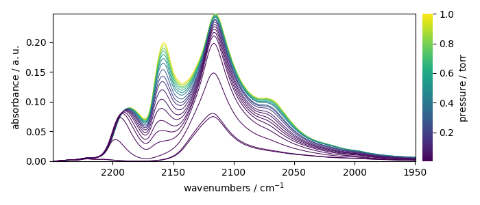
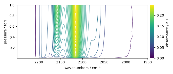
Coord: [float64] torr (size: 19)

IRIS analysis without regularization

Perform IRIS without regularization (the loglevel can be set to INFO to have information on the running process)

iris1 = scp.IRIS(log_level="INFO")

first we compute the kernel object

K = scp.IrisKernel(X_, "langmuir", q=[-8, -1, 50])

Creating Kernel...
Kernel now ready as IrisKernel().kernel!

The actual kernel is given by the kernel attribute

kernel = K.kernel
kernel

NDDataset: [float64] unitless (shape: (y:19, x:50))[langmuir kernel matrix]

Summary

name

:

langmuir kernel matrix

author

:

runner@fv-az2211-104

created

:

2025-04-27 01:43:39+00:00

Data

title

:

coverage

values

:

...

[[ 0.06424 0.1265 ... 0.001332 0.0005778]
[ 0.0659 0.1303 ... 0.00177 0.0007683]
...
[ 0.0714 0.1428 ... 0.1056 0.05078]
[ 0.0714 0.1428 ... 0.1084 0.05227]]

shape

:

(y:19, x:50)

Dimension `x`

size

:

50

title

:

$\Delta_{ads}G^{0}/RT$

coordinates

:

[ -8 -7.857 ... -1.143 -1]

Dimension `y`

size

:

19

title

:

pressure

coordinates

:

[ 0.003 0.004 ... 0.905 1.004] torr

Now we fit the model - we can pass either the Kernel object or the kernel NDDataset

iris1.fit(X_, K)

 Build S matrix (sharpness)
 ... done
 Solving for 312 channels and 19 observations, no regularization
 -->  residuals = 1.09e-01    curvature = 9.14e+04
 Done.

<spectrochempy.analysis.decomposition.iris.IRIS object at 0x7fcff20070e0>

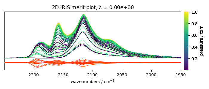
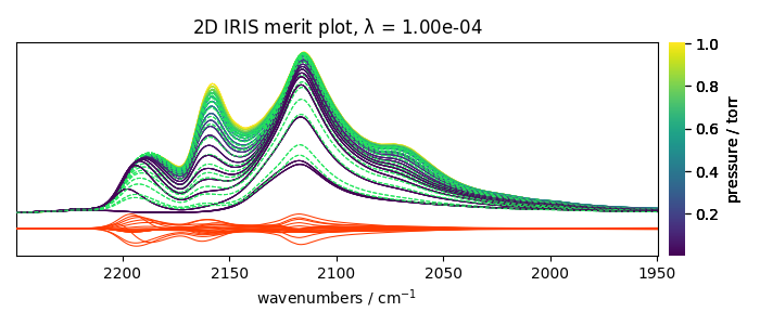
Plots the results

iris1.plotdistribution()
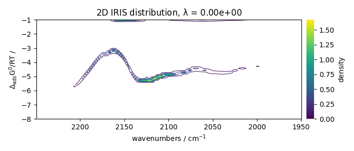
iris1.plotmerit()

• 
• 

[<Matplotlib Axes object>]

With regularization and a manual search

Perform IRIS with regularization, manual search

iris2 = scp.IRIS(reg_par=[-10, 1, 12])

We keep the same kernel object as previously - performs the fit.

iris2.fit(X_, K)
iris2.plotlcurve(title="L curve, manual search")

<Axes: title={'center': 'L curve, manual search'}, xlabel='Residuals', ylabel='Curvature'>

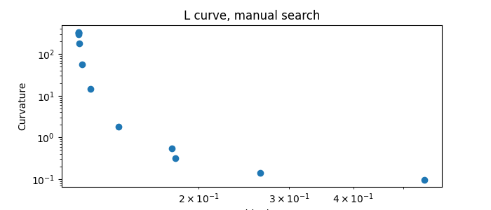
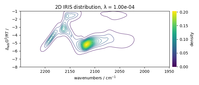
Visually, the best regularization parameter is at index ~ -6, corresponding to lambda = 1e-4

iris2.plotdistribution(-6)
iris2.plotmerit(-6)

• 
• 

[<Matplotlib Axes object>]

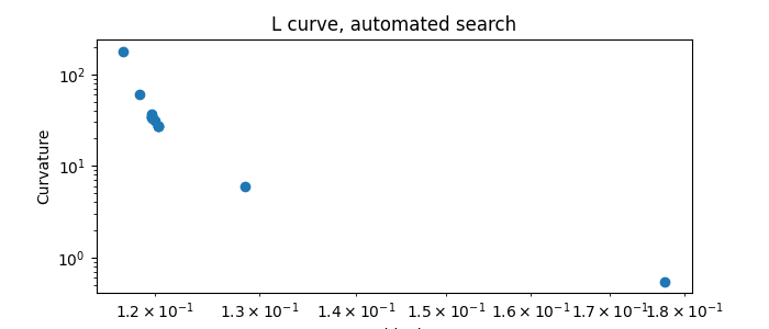
Automatic search

%% Now try an automatic search of the regularization parameter around the best value found manually:

iris3 = scp.IRIS(log_level="INFO", reg_par=[-6, -2])
iris3.fit(X_, K)
iris3.plotlcurve(title="L curve, automated search")

 Build S matrix (sharpness)
 ... done
 Solving for 312 channel(s) and 19 observations, search optimum regularization parameter in the range: [10**-6, 10**-2]
 Initial Log(lambda) values = [      -6   -4.472   -3.528       -2]
 log10(lambda)=-6.000 -->  residuals = 1.171e-01    regularization constraint  = 1.796e+02
 log10(lambda)=-4.472 -->  residuals = 1.203e-01    regularization constraint  = 2.751e+01
 log10(lambda)=-3.528 -->  residuals = 1.286e-01    regularization constraint  = 5.986e+00
 log10(lambda)=-2.000 -->  residuals = 1.773e-01    regularization constraint  = 5.488e-01
 Curvatures of the inner points: C1 = 0.040 ; C2 = 0.105
 New range of Log(lambda) values: [      -6   -5.056   -4.472   -3.528]
 log10(lambda)=-5.056 -->  residuals = 1.186e-01    regularization constraint  = 6.040e+01
 new curvature: C2 = 0.051
 New range (Log lambda):[  -5.056   -4.472   -4.111   -3.528]
 log10(lambda)=-4.111 -->  residuals = 1.223e-01    regularization constraint  = 1.687e+01
 Curvatures of the inner points: C1 = 0.054 ; C2 = 0.047
 New range of Log(lambda) values: [  -5.056   -4.695   -4.472   -4.111]
 log10(lambda)=-4.695 -->  residuals = 1.197e-01    regularization constraint  = 3.702e+01
 new curvature: C2 = 0.091
 New range (Log lambda):[  -4.695   -4.472   -4.334   -4.111]
 log10(lambda)=-4.334 -->  residuals = 1.207e-01    regularization constraint  = 2.273e+01
 Curvatures of the inner points: C1 = -0.020 ; C2 = 0.272
 New range of Log(lambda) values: [  -4.695   -4.557   -4.472   -4.334]
 log10(lambda)=-4.557 -->  residuals = 1.200e-01    regularization constraint  = 3.087e+01
 new curvature: C2 = -0.042
 New range of Log(lambda) values: [  -4.695    -4.61   -4.557   -4.472]
 log10(lambda)=-4.610 -->  residuals = 1.198e-01    regularization constraint  = 3.330e+01
 new curvature: C2 = -0.275
 New range of Log(lambda) values: [  -4.695   -4.642    -4.61   -4.557]
 log10(lambda)=-4.642 -->  residuals = 1.197e-01    regularization constraint  = 3.480e+01
 new curvature: C2 = 0.234
 New range (Log lambda):[  -4.642    -4.61    -4.59   -4.557]
 log10(lambda)=-4.590 -->  residuals = 1.199e-01    regularization constraint  = 3.241e+01
 Curvatures of the inner points: C1 = 0.092 ; C2 = 0.440
 New range of Log(lambda) values: [  -4.642   -4.622    -4.61    -4.59]
 log10(lambda)=-4.622 -->  residuals = 1.197e-01    regularization constraint  = 3.386e+01
 new curvature: C2 = 0.083
 New range (Log lambda): [  -4.642    -4.63   -4.622    -4.61]
 log10(lambda)=-4.630 -->  residuals = 1.197e-01    regularization constraint  = 3.422e+01
  optimum found: index = 5 ; Log(lambda) = -4.622 ; lambda = 2.38602e-05 ; curvature = 0.092
 Done.

<Axes: title={'center': 'L curve, automated search'}, xlabel='Residuals', ylabel='Curvature'>

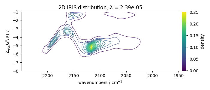
The data corresponding to the largest curvature of the L-curve are at index 5 of the output data.

iris3.plotdistribution(5)
iris3.plotmerit(5)

• 
• 

[<Matplotlib Axes object>]

This ends the example ! The following line can be uncommented if no plot shows when running the .py script with python

# scp.show()