× ⚠️ You are reading the development version documentation.
Read here the documentation of the last stable release.

Denoising

import spectrochempy as scp

SpectroChemPy's API - v.0.8.2.dev7 ©Copyright 2014-2025 - A.Travert & C.Fernandez @ LCS

Denoising 2D spectra

Denoising 2D spectra can be done using the above filtering techniques which can be applied sequentially to each rows of a 2D dataset.

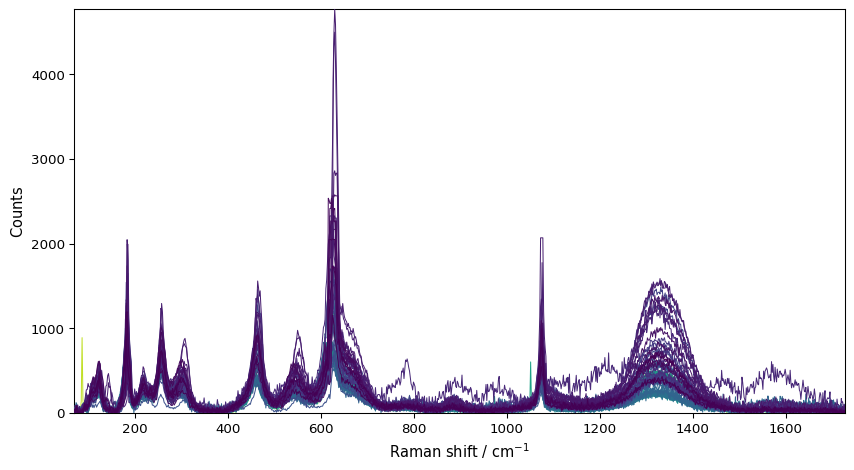
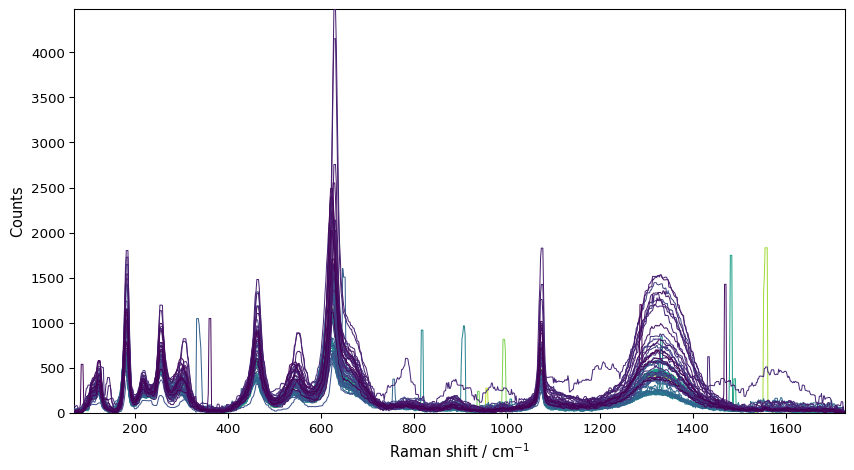
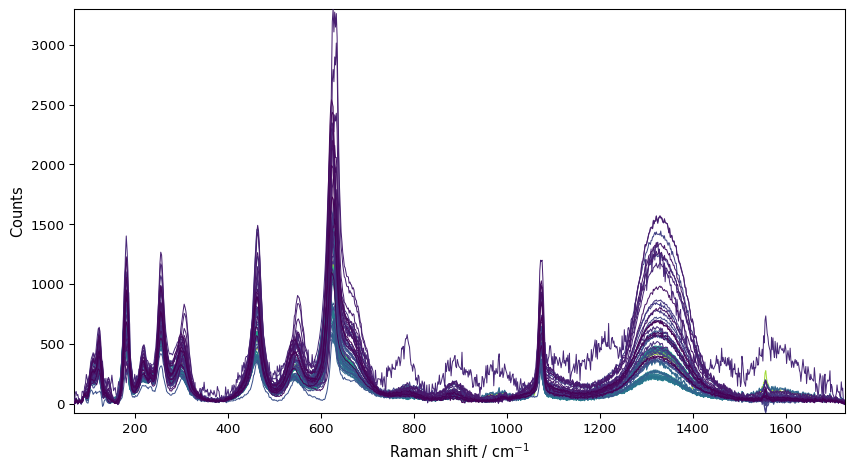
e.g., let’s take a series of Raman spectra for demonstration: These spectra present both a significant noise and cosmic rays spikes.

# Load the data
dataset = scp.read("ramandata/labspec/serie190214-1.txt")
# select the useful region (in particular spectra are 0 after 6500 s)
nd = dataset[0.0:6500.0, 70.0:]
# baseline correction the data (for a easier comparison)
nd1 = nd.snip()
# plot
prefs = scp.preferences
prefs.figure.figsize = (9, 5)
nd1.plot()

Running on GitHub Actions
MPL Configuration directory: /home/runner/.config/matplotlib
Stylelib directory: /home/runner/.config/matplotlib/stylelib

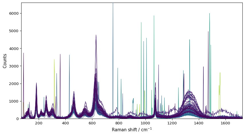
We can apply a Savgol filter to denoise the spectra

nd2 = nd1.savgol(size=7, order=2)
nd2.plot()

The problem is that, not only the spikes are not removed, but they are also broadened.

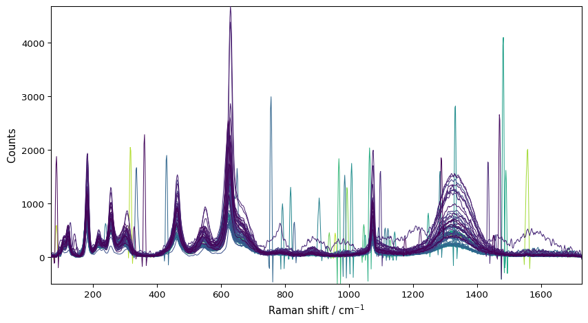
A better way to simply denoise this spectra is to use the denoise dataset method.

The ratio parameter fix the amount of variance we want to preserve in % (default 99.8%)

nd3 = nd1.denoise(ratio=90)
nd3.plot()

This clearly help to increase the signal-to-noise ratio. However, it apparently has in the present case a poor effect on eliminating cosmic ray peaks.

Removing cosmic rays spike from Raman spectra

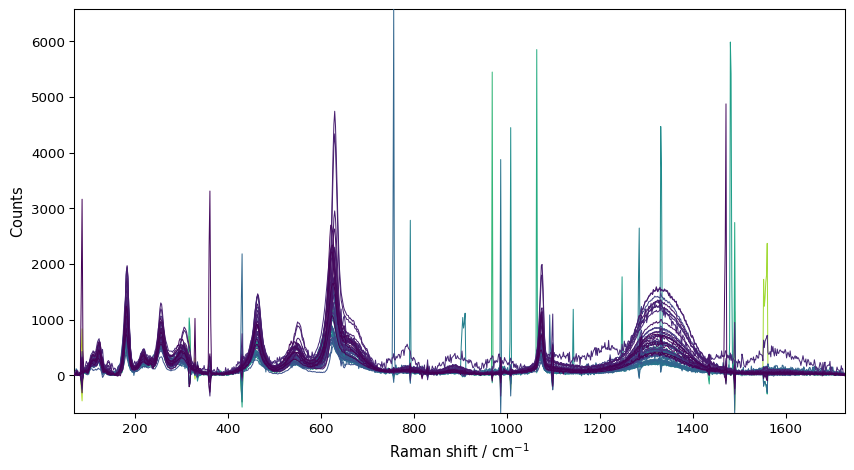
Median filter

A first way to perform this is to apply a median-filter to the data

filter = scp.Filter(method="median", size=5)
nd4 = filter(nd1)
nd4.plot()

However, the spike are not fully removed, and are broadened.

despike method

To obtain better results, one can use the despike methods. The default method (‘katsumo’) is based on :cite:t:katsumoto:2003. The second one (‘whitaker’) is based on :cite:t:Whitaker:2018 For both methods, only two parameters needs to be tuned: delta, a threshold for the detection of spikes, and size the size of the window to consider around the spike to estimate the original intensity.

X = nd1[0]
nd5 = scp.despike(X, size=11, delta=5)
X.plot()
nd5.plot(clear=False, ls="-", c="r")

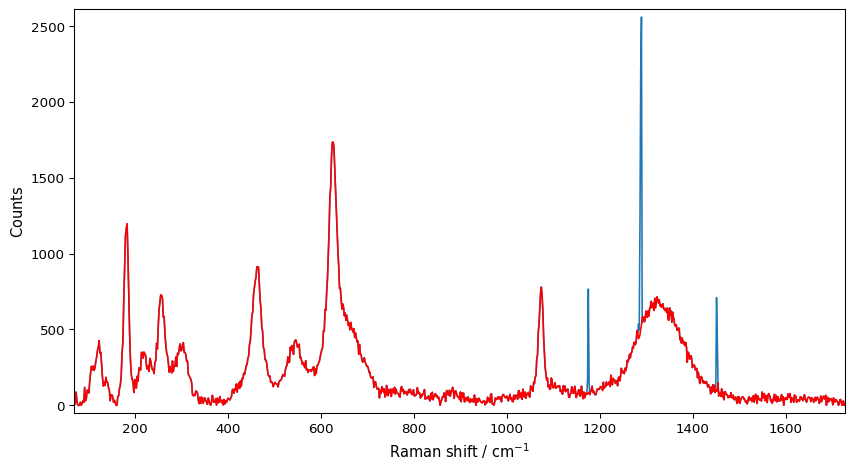
Getting the desired results require the tuning of size and delta parameters. And sometimes may need to repeat the procedure on a previously filtered spectra.

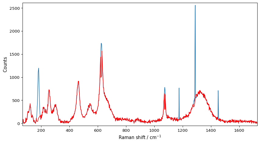
For example, it size or delta are badly chosen, valid peaks could be removed. So careful inspection of the results is crucial.

nd5b = scp.despike(X, size=21, delta=2)
X.plot()
nd5b.plot(clear=False, ls="-", c="r")

Last we can apply it to the full 2D dataset

nd6 = scp.despike(nd1, size=11, delta=5)
nd6.plot()

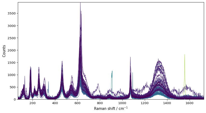
It is however rarely perfect as the setting of size and delta may be depending on the row.

A possibility to improve it is to apply a denoise filter afterward.

nd7 = nd6.denoise(ratio=92)
nd7.plot()

The ‘whitaker’ method is also available:

nd8 = scp.despike(nd1, size=11, delta=5, method="whitaker")
nd8.plot()