× ⚠️ You are reading the development version documentation.
Read here the documentation of the last stable release.

Solve a linear equation using LSTSQ

In this example, we find the least square solution of a simple linear equation.

import spectrochempy as scp

Prepare example data

Noisy distance-vs-time measurements:

time = [0, 1, 2, 3]
distance = [-1, 0.2, 0.9, 2.1]

Using plain arrays (or lists)

Fit a linear model distance = v * time + d0:

lstsq = scp.LSTSQ()
_ = lstsq.fit(time, distance)
v = lstsq.coef
d0 = lstsq.intercept
rsquare = lstsq.score()
v, d0, rsquare

(0.9999999999999997, np.float64(-0.9499999999999995), 0.9900990099009901)

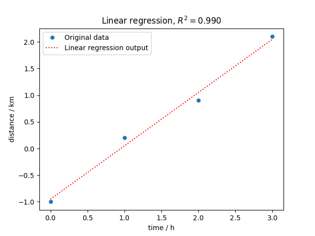
Plot the result:

import matplotlib.pyplot as plt

_ = plt.plot(time, distance, "o", label="Original data", markersize=5)
distance_fitted = lstsq.predict()
_ = plt.plot(time, distance_fitted, ":r", label="Linear regression output")
plt.xlabel("time / h")
plt.ylabel("distance / km")
plt.title(f"Linear regression, $R^2={rsquare:.3f}$")
plt.legend()

<matplotlib.legend.Legend object at 0x7f41d61e6e90>

Using NDDatasets as input (X and Y)

NDDatasets carry metadata such as units:

time = scp.NDDataset([0, 1, 2, 3], title="time", units="hour")
distance = scp.NDDataset([-1, 0.2, 0.9, 2.1], title="distance", units="kilometer")

Fit and inspect the results (now with units):

lstsq = scp.LSTSQ()
_ = lstsq.fit(time, distance)

v = lstsq.coef
d0 = lstsq.intercept
rsquare = lstsq.score()
print(f"speed : {v: .2f},  d0 : {d0: .2f},  r^2={rsquare: .3f}")

speed :  1.00 kilometer hour^-1,  d0 : -0.95 kilometer,  r^2= 0.990

Prediction returns an NDDataset when inputs are NDDatasets:

distance_fitted2 = lstsq.predict()
print(distance_fitted2)

assert (distance_fitted == distance_fitted2.data).all()

NDDataset: [float64] km (size: 4)

Using a single NDDataset with x-coordinates

The x-coordinate of the NDDataset is used as the predictor:

time = scp.Coord([0, 1, 2, 3], title="time", units="hour")
distance = scp.NDDataset(
    data=[-1, 0.2, 0.9, 2.1], coordset=[time], title="distance", units="kilometer"
)

Fit using only the NDDataset (the x-coordinate provides the time axis):

lstsq = scp.LSTSQ()
_ = lstsq.fit(distance)

v = lstsq.coef
d0 = lstsq.intercept
rsquare = lstsq.score()
print(f"speed : {v:.2f~C},  d0 : {d0:.2f~C},  r^2={rsquare:.3f}")

speed : 1.00 km*h**-1,  d0 : -0.95 km,  r^2=0.990

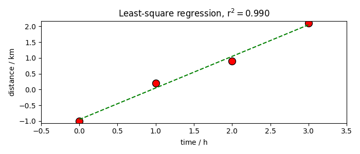
Final plot using the dataset’s own plot methods:

_ = distance.plot_scatter(
    markersize=10,
    mfc="red",
    mec="black",
    label="Original data",
    title=f"Least-square regression, $r^2={rsquare:.3f}$",
)
distance_fitted3 = lstsq.predict()
_ = distance_fitted3.plot_pen(clear=False, color="g", label="Fitted line", legend=True)

This ends the example ! The following line can be uncommented if no plot shows when running the .py script with python

# scp.show()