× ⚠️ You are reading the development version documentation.
Read here the documentation of the last stable release.

EFA example

In this example, we perform the Evolving Factor Analysis

sphinx_gallery_thumbnail_number = 2

import os

import spectrochempy as scp

Load and preprocess the dataset

datadir = scp.preferences.datadir
dataset = scp.read_omnic(os.path.join(datadir, "irdata", "nh4y-activation.spg"))

Change the time origin

dataset.y -= dataset.y[0]

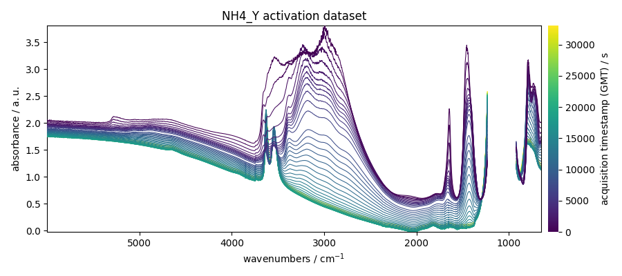
Mask saturated regions and preview

dataset[:, 1230.0:920.0] = scp.MASKED  # do not forget to use float in slicing
dataset[:, 5997.0:5993.0] = scp.MASKED

_ = dataset.plot_stack(title="NH4_Y activation dataset")

Fit the EFA model

efa1 = scp.EFA()
_ = efa1.fit(dataset)

Forward and backward evolution

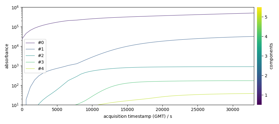
Forward evolution of the first 5 components

f = efa1.f_ev[:, :5]
_ = f.T.plot(yscale="log", legend=f.k.labels)

Note the use of coordinate k (component axis) in the expression above. To find the actual names of the coordinates, use the dims attribute:

f.dims

['y', 'k']

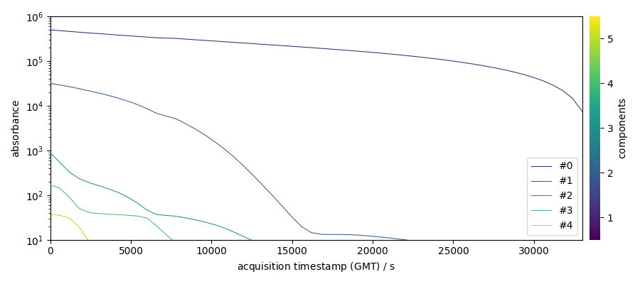
Backward evolution

b = efa1.b_ev[:, :5]
_ = b.T[:5].plot(yscale="log", legend=b.k.labels)

Select the number of components and extract concentrations

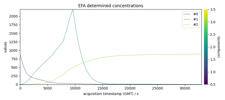
Use 3 components (the 4th component magnitude serves as the noise cutoff):

efa1.n_components = 3
efa1.cutoff = efa1.f_ev[:, 3].max()

C1 = efa1.transform()
_ = C1.T.plot(title="EFA determined concentrations", legend=C1.k.labels)

The same can be done in one step with fit_transform:

efa2 = scp.EFA(n_components=3)
C2 = efa2.fit_transform(dataset)
assert C1 == C2

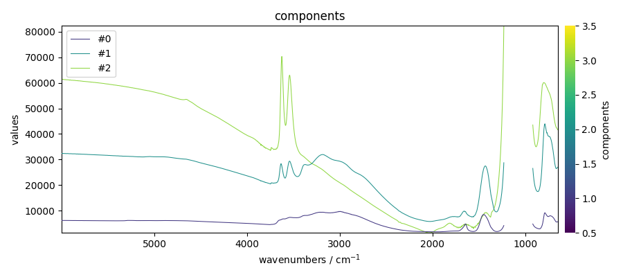
Extract the resolved components

St = efa2.get_components()
_ = St.plot(title="components", legend=St.k.labels)

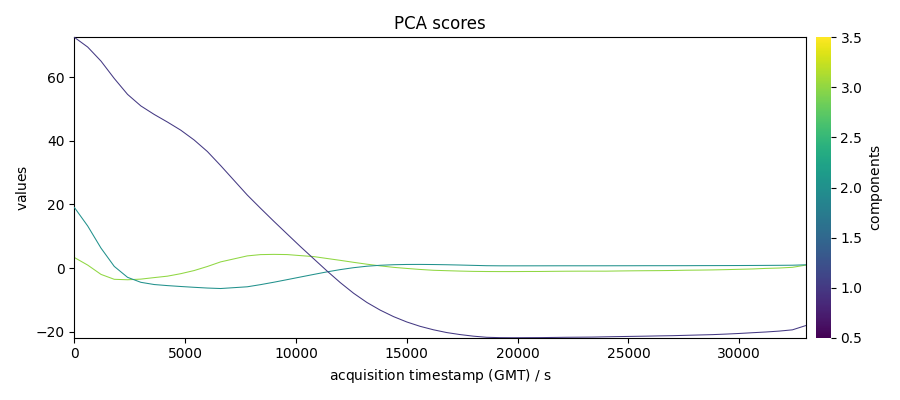
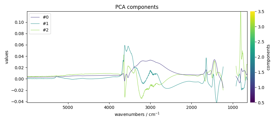
Compare with PCA

pca = scp.PCA(n_components=3)
C3 = pca.fit_transform(dataset)

_ = C3.T.plot(title="PCA scores")

LT = pca.loadings
_ = LT.plot(title="PCA components", legend=LT.k.labels)

This ends the example ! The following line can be uncommented if no plot shows when running the .py script with python

# scp.show()