× ⚠️ You are reading the development version documentation.
Read here the documentation of the last stable release.

Processing a saturation-recovery relaxation series

This example processes a pseudo-2D series of 1D spectra acquired with a variable recovery delay and fits a simple saturation-recovery model to the dominant resonance.

The bundled Bruker dataset stores the delays in vdlist and the pulse program indicates a CP/MAS saturation-recovery experiment. The example keeps a modest public scope:

• process the 1D FIDs with explicit SpectroChemPy operations;

• extract a signal trace from the dominant processed resonance;

• fit a simple two-parameter recovery model to that trace.

It does not claim replay of vendor processing, nor exact equivalence with the TopSpin fitting tools bundled alongside the dataset.

Requires the official spectrochempy-nmr plugin. Install with: pip install spectrochempy[nmr].

Import API

import spectrochempy as scp

# short version of the unit registry
U = scp.ur

Import a pseudo-2D delay series

Define the folder containing the Bruker experiment.

datadir = scp.preferences.datadir
nmrdir = datadir / "nmrdata" / "bruker" / "tests" / "nmr"

dataset = scp.nmr.read(nmrdir / "relax" / "100" / "ser", use_list="vdlist")

Analysing the data

Print dataset summary

dataset

NDDataset [relax expno:100 procno:1 (SER)] — complex128, shape: (y:9, x:1982), count

name

:

relax expno:100 procno:1 (SER)

author

:

runner@runnervmzvulz

created

:

2026-08-13 17:04:33+00:00

history

:

2026-08-13 17:04:33+00:00> Imported from TopSpin dataset

Data

title

:

intensity

values

:

R[[ 0.5522 2.137 ... -1.437 -0.02603]
[ 1.099 3.404 ... -0.6497 -0.0129]
...
[ 1.603 5.99 ... 4.959 0.09235]
[ 1.61 6.14 ... -0.7725 -0.01501]] countI[[ -1.513 -2.733 ... 4.471 0.08437]
[ -2.496 -4.623 ... -6.003 -0.1152]
...
[ -4.25 -7.726 ... 4.695 0.08693]
[ -4.302 -7.69 ... 0.222 0.004867]] count

shape

:

(y:9, x:1982(complex))

Dimension `x`

size

:

1982

title

:

F2 acquisition time

coordinates

:

[ 0 6.4 ... 1.267e+04 1.268e+04] µs

Dimension `y`

size

:

9

title

:

time

coordinates

:

[ 1 2 ... 20 50] s

Plot the processed spectra

The vdlist delays become the secondary coordinate of the pseudo-2D series.

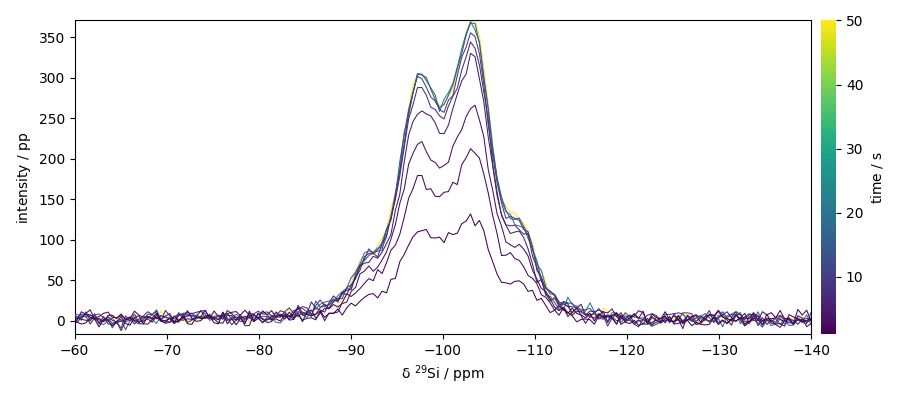
ds = dataset.em(lb=15 * U.Hz)
ds = ds.fft()
ds = ds.pk(phc0=-145 * U.deg, phc1=0 * U.deg)
_ = ds.plot(xlim=(100, -50))

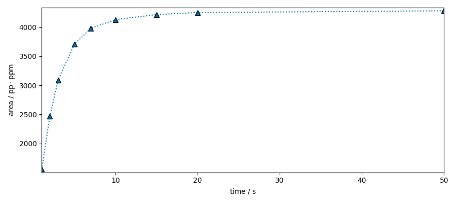
Build a signal trace from the dominant resonance

The strongest processed peak in this series sits around 20–22 ppm. We integrate a narrow ppm window around that resonance for each delay.

signal = ds[:, 20.0:45.0].simpson()
_ = signal.plot(marker="^", ls=":")
signal.real

NDDataset [relax expno:100 procno:1 (SER)] — float64, size: 9, count⋅ppm

name

:

relax expno:100 procno:1 (SER)

author

:

runner@runnervmzvulz

created

:

2026-08-13 17:04:33+00:00

description

:

Integration of NDDataset 'relax expno:100 procno:1 (SER)' along dim: 'x'.

history

:

2026-08-13 17:04:33+00:00> Dataset resulting from application of `simpson` method

Data

title

:

area

values

:

[ 1512 2565 ... 4203 4328] count⋅ppm

size

:

9

Dimension `y`

size

:

9

title

:

time

coordinates

:

[ 1 2 ... 20 50] s

Fit a model

create an Optimize object using a simple leastsq method

fitter = scp.Optimize(log_level="INFO", method="leastsq")

Define the model to fit

def T1_model(t, I0, T1):  # no underscore in parameters names.
    # Simple saturation-recovery model.
    import numpy as np

    I = I0 * (1 - np.exp(-t / T1))
    return I

Add the model to the fitter usermodels as it it not a built-in model

fitter.usermodels = {"T1_model": T1_model}

Define the parameter variables using a script (parameter: value, low_bound, high_bound) no underscore in parameters names.

fitter.script = """
MODEL: T1
shape: T1_model
  $ I0:  1000.0, 1, none
  $ T1:  2.0,    0.1, none
"""

Perform the fit

_ = fitter.fit(signal)

som = fitter.predict()
som

NDDataset [relax expno:100 procno:1 (SER)_Optimize.fitted_data] — float64, shape: (u:1, y:9), count⋅ppm

name

:

relax expno:100 procno:1 (SER)_Optimize.fitted_data

author

:

runner@runnervmzvulz

created

:

2026-08-13 17:04:33+00:00

description

:

Fitted data from Optimize fit of relax expno:100 procno:1 (SER).

history

:

2026-08-13 17:04:33+00:00> Created fitted data with Optimize from relax expno:100 procno:1 (SER).

Data

title

:

fitted data

values

:

[[ 1513 2483 ... 4219 4219]] count⋅ppm

shape

:

(u:1, y:9)

Dimension `u`

title

:

coordinates

:

Undefined

Dimension `y`

size

:

9

title

:

time

coordinates

:

[ 1 2 ... 20 50] s

Plot the measured recovery points and the fitted curve separately so the experimental series remains a true scatter plot.

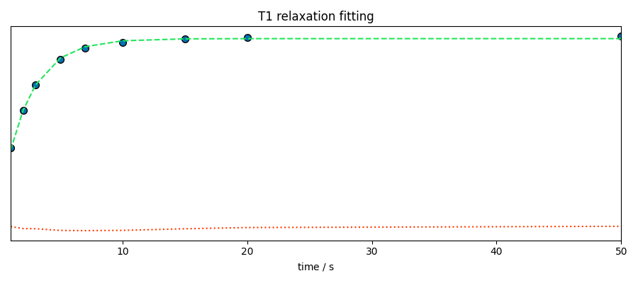
ax = signal.plot_scatter(
    color="tab:blue",
    marker="o",
    markersize=5,
    label="measured signal",
    title="Saturation-recovery fit of the dominant resonance",
)
_ = som.plot(clear=False, color="tab:orange", lw=1.8, label="fitted curve")
_ = ax.legend()

This ends the example ! The following line can be removed or commented when the example is run as a notebook (ipynb).

# scp.show()