× ⚠️ You are reading the development version documentation.
Read here the documentation of the last stable release.

MCR-ALS with kinetic constraints

In this example, we perform the MCR ALS optimization of the UV-vis of spectra resulting from a three-component reaction A -> B -> C which was investigated by UV–Vis spectroscopy. Full details on the reaction and data acquisition conditions can be found in Bijlsma et al. [2001] . The data can be downloded from the author website Biosystems Data Analysis group University of Amsterdam (Copyright 2005 Biosystems Data Analysis Group ; Universiteit van Amsterdam ). For the user convenience, # this dataset is present in the ‘datadir’ of spectrochempy in ‘matlabdata/METING9.MAT’.

import numpy as np

import spectrochempy as scp

Loading a NDDataset

Load the data with the read function.

ds = scp.read("matlabdata/METING9.MAT")

This file contains a pair of datasets. The first dataset contains the time in seconds since the start of the reaction (t=0). The second dataset contains the UV-VIS spectra of the reaction mixture, recorded at different time points. The first column of the matrix contains the wavelength axis and the remaining columns are the measured UV-VIS spectra (wavelengths x timepoints)

print("NDDataset names: " + str([d.name for d in ds]))

NDDataset names: ['RelTime', 'x9b']

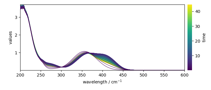
We load the experimental spectra (in ds[1]), add the y (time) and x (wavelength) coordinates, and keep one spectrum of out 4:

D = scp.NDDataset(ds[1][:, 1:].data.T)
D.y = scp.Coord(ds[0].data.squeeze(), title="time") / 60
D.x = scp.Coord(ds[1][:, 0].data.squeeze(), title="wavelength / cm$^{-1}$")
D = D[::4]
D.plot()

A first estimate of the concentrations can be obtained by EFA:

print("compute EFA...")
efa = scp.EFA()
efa.fit(D[:, 300.0:500.0])
efa.n_components = 3
C0 = efa.transform()
C0 = C0 / C0.max(dim="y") * 5.0
C0.T.plot()

compute EFA...

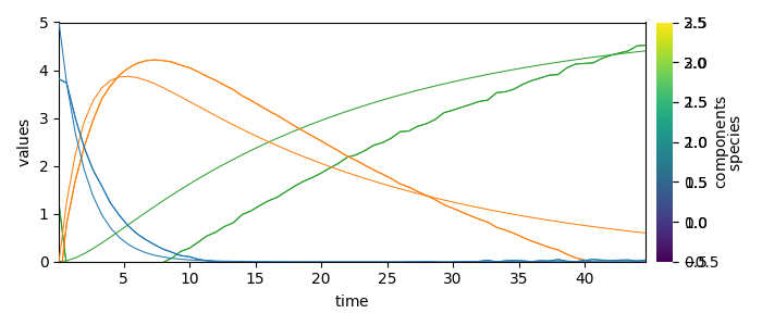
We can get a better estimate of the concentration (C) and pure spectra profiles (St) by soft MCR-ALS:

mcr_1 = scp.MCRALS(log_level="INFO")
mcr_1.fit(D, C0)
mcr_1.C.T.plot()
mcr_1.St.plot()

• 
• 

Concentration profile initialized with 3 components
Initial spectra profile computed
***           ALS optimisation log            ***
#iter     RSE / PCA        RSE / Exp      %change
-------------------------------------------------
  1        0.002867        0.005886      -99.284101
  2        0.002813        0.005863       -0.390168
  3        0.002810        0.005861       -0.020846
converged !

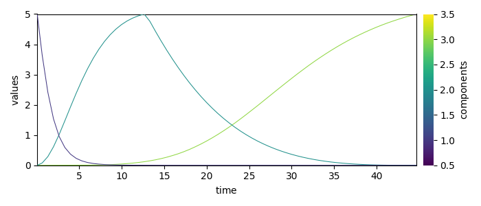
Kinetic constraints can be added, i.e., imposing that the concentration profiles obey a kinetic model. To do so we first define an ActionMAssKinetics object with roughly estimated rate constants:

reactions = ("A -> B", "B -> C")
species_concentrations = {"A": 5.0, "B": 0.0, "C": 0.0}
k0 = np.array((0.5, 0.05))
kin = scp.ActionMassKinetics(reactions, species_concentrations, k0)

The concentration profile obtained with this approximate model can be computed and compared with those of the soft MCR-ALS:

Ckin = kin.integrate(D.y.data)
mcr_1.C.T.plot(linestyle="-", cmap=None)
Ckin.T.plot(clear=False, cmap=None)

Even though very approximate, the same values can be used to run a hard-soft MCR-ALS:

X = D[:, 300.0:500.0]
param_to_optimize = {"k[0]": 0.5, "k[1]": 0.05}
mcr_2 = scp.MCRALS()
mcr_2.hardConc = [0, 1, 2]
mcr_2.getConc = kin.fit_to_concentrations
mcr_2.argsGetConc = ([0, 1, 2], [0, 1, 2], param_to_optimize)
mcr_2.kwargsGetConc = {"ivp_solver_kwargs": {"return_NDDataset": False}}

mcr_2.fit(X, Ckin)

Optimization terminated successfully.
         Current function value: 0.000000
         Iterations: 17
         Function evaluations: 35
Optimization terminated successfully.
         Current function value: 4.004007
         Iterations: 27
         Function evaluations: 54
Optimization terminated successfully.
         Current function value: 2.293919
         Iterations: 23
         Function evaluations: 45
Optimization terminated successfully.
         Current function value: 1.749865
         Iterations: 22
         Function evaluations: 43
Optimization terminated successfully.
         Current function value: 1.403400
         Iterations: 22
         Function evaluations: 43

<spectrochempy.analysis.decomposition.mcrals.MCRALS object at 0x7fcfddae1bd0>

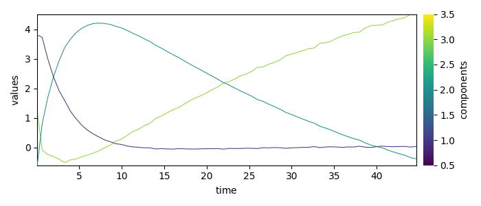
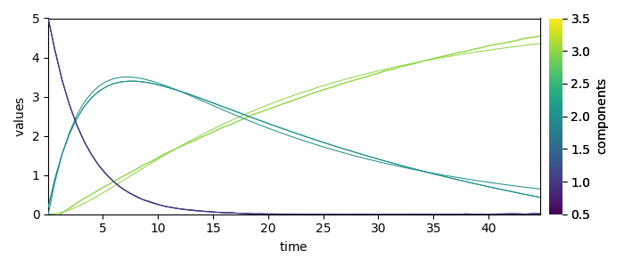
Now, let’s compare the concentration profile of MCR-ALS (C = X(C_{kin}^+ X)^+) with that of the optimized kinetic model (C_{kin} equiv C_constrained):

mcr_2.C.T.plot()
mcr_2.C_constrained.T.plot(clear=False)

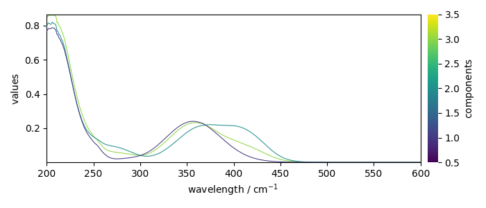
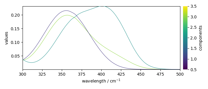
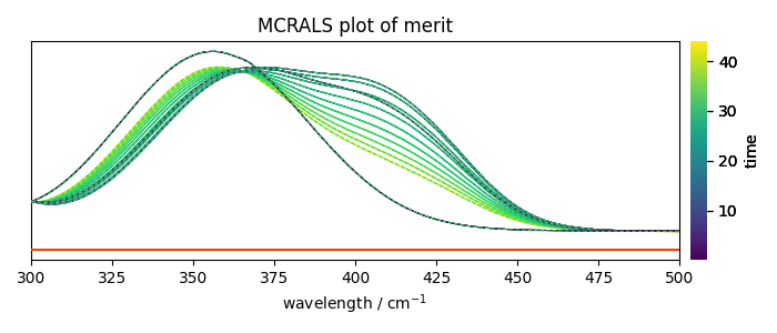
Finally, let’s plot some of the pure spectra profiles St, and the

reconstructed dataset (X_hat = C St) vs original dataset (X) and residuals.

mcr_2.St.plot()
mcr_2.plotmerit(nb_traces=10)

• 
• 

This ends the example ! The following line can be uncommented if no plot shows when running the .py script with python

# scp.show()