spectrochempy.PCA

class PCA(*, log_level='WARNING', warm_start=False, iterated_power='auto', n_components=None, n_oversamples=10, power_iteration_normalizer='auto', random_state=None, scaled=False, standardized=False, svd_solver='auto', tol=0.0, whiten=False)[source]

Principal Component Anamysis (PCA).

The Principal Component Analysis analysis is using the sklearn.decomposition.PCA model.

Parameters:

log_level (any of ["INFO", "DEBUG", "WARNING", "ERROR"], optional, default: "WARNING") – The log level at startup. It can be changed later on using the set_log_level method or by changing the log_level attribute.
warm_start (bool, optional, default: False) – When fitting repeatedly on the same dataset, but for multiple parameter values (such as to find the value maximizing performance), it may be possible to reuse previous model learned from the previous parameter value, saving time.

When warm_start is True, the existing fitted model attributes is used to initialize the new model in a subsequent call to fit.
iterated_power (an int or any of [‘auto’], optional, default: 'auto') – Number of iterations for the power method computed by svd_solver == ‘randomized’. Must be of range [0, infinity).
n_components (any of [‘mle’] or an int or a float, optional, default: None) – Number of components to keep. if n_components is not set all components are kept:
```
n_components == min(n_observations, n_features)
```
If n_components == 'mle' and svd_solver == 'full' , Minka’s MLE is used to guess the dimension. Use of n_components == 'mle' will interpret svd_solver == 'auto' as svd_solver == 'full' . If 0 < n_components < 1 and svd_solver == 'full' , select the number of components such that the amount of variance that needs to be explained is greater than the percentage specified by n_components. If svd_solver == 'arpack' , the number of components must be strictly less than the minimum of n_features and n_observations. Hence, the None case results in:
```
n_components == min(n_observations, n_features) - 1.
```
n_oversamples (int, optional, default: 10) – This parameter is only relevant when svd_solver="randomized" . It corresponds to the additional number of random vectors to sample the range of X so as to ensure proper conditioning. See randomized_svd for more details.
power_iteration_normalizer (any value of [ 'auto' , 'QR' , 'LU' , 'none' ], optional, default: 'auto') – Power iteration normalizer for randomized SVD solver. Not used by ARPACK. See randomized_svd for more details.
random_state (an int or a RandomState, optional, default: None) – Used when the ‘arpack’ or ‘randomized’ solvers are used. Pass an int for reproducible results across multiple function calls.
scaled (bool, optional, default: False) – If True the data are scaled in the interval [0-1]: \(X' = (X - min(X)) / (max(X)-min(X))\).
standardized (bool, optional, default: False) – If True the data are scaled to unit standard deviation: \(X' = X / \sigma\).
svd_solver (any value of [ 'auto' , 'full' , 'arpack' , 'randomized' ], optional, default: 'auto') – If auto : The solver is selected by a default policy based on X.shape and n_components: if the input data is larger than 500x500 and the number of components to extract is lower than 80% of the smallest dimension of the data, then the more efficient ‘randomized’ method is enabled. Otherwise the exact full SVD is computed and optionally truncated afterwards. If full : run exact full SVD calling the standard LAPACK solver via scipy.linalg.svd and select the components by postprocessing If arpack : run SVD truncated to n_components calling ARPACK solver via scipy.sparse.linalg.svds . It requires strictly 0 < n_components < min(X.shape) If randomized : run randomized SVD by the method of Halko et al.
tol (float, optional, default: 0.0) – Tolerance for singular values computed by svd_solver == ‘arpack’. Must be of range [0.0, infinity).
whiten (bool, optional, default: False) – When True (False by default) the components_ vectors are multiplied by the square root of n_observations and then divided by the singular values to ensure uncorrelated outputs with unit component-wise variances. Whitening will remove some information from the transformed signal (the relative variance scales of the components) but can sometime improve the predictive accuracy of the downstream estimators by making their data respect some hard-wired assumptions.

See also

EFA: Perform an Evolving Factor Analysis (forward and reverse).
FastICA: Perform Independent Component Analysis with a fast algorithm.
IRIS: Integral inversion solver for spectroscopic data.
MCRALS: Perform MCR-ALS of a dataset knowing the initial \(C\) or \(S^T\) matrix.
NMF: Non-Negative Matrix Factorization.
SIMPLISMA: SIMPLe to use Interactive Self-modeling Mixture Analysis.
SVD: Perform a Singular Value Decomposition.

Initialize the BaseConfigurable class.

Parameters:

log_level (int, optional) – The log level at startup. Default is logging.WARNING.
**kwargs (dict) – Additional keyword arguments for configuration.

Attributes Summary

`X`	Return the X input dataset (eventually modified by the model).
`Y`	The `Y` input.
`components`	`NDDataset` with components in feature space (n_components, n_features).
`config`	`traitlets.config.Config` object.
`iterated_power`	Number of iterations for the power method computed by svd_solver == 'randomized'.
`loadings`	Return PCA loadings.
`log`	Return `log` output.
`n_components`	Number of components to keep. if `n_components` is not set all components are kept::.
`n_oversamples`	This parameter is only relevant when `svd_solver="randomized"` .
`name`	Object name
`power_iteration_normalizer`	Power iteration normalizer for randomized SVD solver.
`random_state`	Used when the 'arpack' or 'randomized' solvers are used.
`scaled`	\(X' = (X - min(X)) / (max(X)-min(X))\).
`scores`	Returns PCA scores.
`standardized`	\(X' = X / \sigma\).
`svd_solver`	If auto: The solver is selected by a default policy based on `X.shape` and `n_components`: if the input data is larger than 500x500 and the number of components to extract is lower than 80% of the smallest dimension of the data, then the more efficient 'randomized' method is enabled.
`tol`	Tolerance for singular values computed by svd_solver == 'arpack'.
`whiten`	When True (False by default) the `components_` vectors are multiplied by the square root of n_observations and then divided by the singular values to ensure uncorrelated outputs with unit component-wise variances.

Methods Summary

`fit`(X)	Fit the PCA model on X.
`fit_transform`(X[, Y])	Fit the model with `X` and apply the dimensionality reduction on `X`.
`get_components`([n_components])	Return the component's dataset: (selected n_components, n_features).
`inverse_transform`([X_transform])	Transform data back to its original space.
`parameters`([replace, removed, default])	Alias for `params` method.
`params`([default])	Return current or default configuration values.
`plot_merit`([X, X_hat])	Plot the input (`X`), reconstructed (`X_hat`) and residuals.
`plot_score`([scores, components])	2D or 3D score plot of observations.
`plot_scree`([n_components])	Scree plot of explained variance + cumulative variance by PCA.
`plotmerit`([X, X_hat])	Plot the input (`X`), reconstructed (`X_hat`) and residuals.
`printev`([n_components])	Print PCA figures of merit.
`reconstruct`([X_transform])	Transform data back to its original space.
`reduce`([X])	Apply dimensionality reduction to `X`.
`reset`()	Reset configuration parameters to their default values.
`scoreplot`(self, args, *kwargs)	2D or 3D scoreplot of observations.
`screeplot`([n_components])	Scree plot of explained variance + cumulative variance by PCA.
`to_dict`()	Return config value in a dict form.
`transform`([X])	Apply dimensionality reduction to `X`.

Attributes Documentation

X: Return the X input dataset (eventually modified by the model).

Y: The Y input.

components

NDDataset with components in feature space (n_components, n_features).

See also

get_components: Retrieve only the specified number of components.

config: traitlets.config.Config object.

iterated_power: Number of iterations for the power method computed by svd_solver == ‘randomized’. Must be of range [0, infinity).

loadings: Return PCA loadings.

log: Return log output.

n_components

Number of components to keep. if n_components is not set all components are kept:

n_components == min(n_observations, n_features)

If n_components == 'mle' and svd_solver == 'full' , Minka’s MLE is used to guess the dimension. Use of n_components == 'mle' will interpret svd_solver == 'auto' as svd_solver == 'full' . If 0 < n_components < 1 and svd_solver == 'full' , select the number of components such that the amount of variance that needs to be explained is greater than the percentage specified by n_components. If svd_solver == 'arpack' , the number of components must be strictly less than the minimum of n_features and n_observations. Hence, the None case results in:

n_components == min(n_observations, n_features) - 1.

n_oversamples: This parameter is only relevant when svd_solver="randomized" . It corresponds to the additional number of random vectors to sample the range of X so as to ensure proper conditioning. See randomized_svd for more details.

name: Object name

power_iteration_normalizer: Power iteration normalizer for randomized SVD solver. Not used by ARPACK. See randomized_svd for more details.

random_state: Used when the ‘arpack’ or ‘randomized’ solvers are used. Pass an int for reproducible results across multiple function calls.

scaled

\(X' = (X - min(X)) / (max(X)-min(X))\).

Type:: If True the data are scaled in the interval [0-1]

scores: Returns PCA scores.

standardized

\(X' = X / \sigma\).

Type:: If True the data are scaled to unit standard deviation

svd_solver: If auto: The solver is selected by a default policy based on X.shape and n_components: if the input data is larger than 500x500 and the number of components to extract is lower than 80% of the smallest dimension of the data, then the more efficient ‘randomized’ method is enabled. Otherwise the exact full SVD is computed and optionally truncated afterwards. If full : run exact full SVD calling the standard LAPACK solver via scipy.linalg.svd and select the components by postprocessing If arpack : run SVD truncated to n_components calling ARPACK solver via scipy.sparse.linalg.svds . It requires strictly 0 < n_components < min(X.shape) If randomized : run randomized SVD by the method of Halko et al.

tol: Tolerance for singular values computed by svd_solver == ‘arpack’. Must be of range [0.0, infinity).

whiten: When True (False by default) the components_ vectors are multiplied by the square root of n_observations and then divided by the singular values to ensure uncorrelated outputs with unit component-wise variances. Whitening will remove some information from the transformed signal (the relative variance scales of the components) but can sometime improve the predictive accuracy of the downstream estimators by making their data respect some hard-wired assumptions.

Methods Documentation

fit(X)[source]

Fit the PCA model on X.

Parameters:: X (NDDataset or array-like of shape (n_observations, n_features)) – Training data.
Returns:: self – The fitted instance itself.

See also

fit_transform: Fit the model with an input dataset X and apply the dimensionality reduction on X.
fit_reduce: Alias of fit_transform (Deprecated).

fit_transform(X, Y=None, **kwargs)[source]

Fit the model with X and apply the dimensionality reduction on X.

Parameters:

X (NDDataset or array-like of shape (n_observations, n_features)) – Training data.
Y (any) – Depends on the model.
**kwargs (keyword parameters, optional) – See Other Parameters.

Returns:

NDDataset – Dataset with shape (n_observations, n_components).

Other Parameters:

n_components (int, optional) – The number of components to use for the reduction. If not given the number of components is eventually the one specified or determined in the fit process.

get_components(n_components=None)

Return the component’s dataset: (selected n_components, n_features).

Parameters:: n_components (int, optional, default: None) – The number of components to keep in the output dataset. If None, all calculated components are returned.
Returns:: NDDataset – Dataset with shape (n_components, n_features)

inverse_transform(X_transform=None, **kwargs)

Transform data back to its original space.

In other words, return an input X_original whose reduce/transform would be X_transform.

Parameters:

X_transform (array-like of shape (n_observations, n_components), optional) – Reduced X data, where n_observations is the number of observations and n_components is the number of components. If X_transform is not provided, a transform of X provided in fit is performed first.
**kwargs (keyword parameters, optional) – See Other Parameters.

Returns:

NDDataset – Dataset with shape (n_observations, n_features).

Other Parameters:

n_components (int, optional) – The number of components to use for the reduction. If not given the number of components is eventually the one specified or determined in the fit process.

See also

reconstruct: Alias of inverse_transform (Deprecated).

parameters(replace="params", removed="0.8.0") def parameters(self, default=False)[source]: Alias for params method.

Deprecated since version 0.8.0: Use params instead.

params(default=False)[source]

Return current or default configuration values.

Parameters:: default (bool, optional, default: False) – If default is True, the default parameters are returned, else the current values.
Returns:: dict – Current or default configuration values.

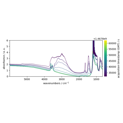
plot_merit(X=None, X_hat=None, **kwargs)[source]

Plot the input (X), reconstructed (X_hat) and residuals.

\(X\) and \(\hat{X}\) can be passed as arguments. If not, the X attribute is used for \(X`and :math:\)hat{X}`is computed by the inverse_transform method

Parameters:

X (NDDataset, optional) – Original dataset. If is not provided (default), the X attribute is used and X_hat is computed using inverse_transform.
X_hat (NDDataset, optional) – Inverse transformed dataset. if X is provided, X_hat must also be provided as compuyed externally.

Returns:

Axes – Matplotlib subplot axe.

Other Parameters:

exp_c (color, colormap, or list of colors, optional) – Color(s) for experimental spectra. - None: use unified semantic resolver (auto-detect categorical/sequential) - Single color: use for all experimental spectra - Colormap name/object: sample colors from colormap - List/tuple: use as explicit color cycle
calc_c (color, colormap, or list of colors, optional) – Color(s) for calculated spectra. - None: use default blue “#2a6fbb” - Single color: use for all calculated spectra - Colormap name/object: sample colors from colormap - List/tuple: use as explicit color cycle
resid_c (color, colormap, or list of colors, optional) – Color(s) for residual spectra. - None: use default grey “0.4” - Single color: use for all residual spectra - Colormap name/object: sample colors from colormap - List/tuple: use as explicit color cycle
exp_linestyle (str, optional) – Line style for experimental spectra. Default: “-“.
calc_linestyle (str, optional) – Line style for calculated spectra. Default: “–“.
resid_linestyle (str, optional) – Line style for residual spectra. Default: “-“.
exp_linewidth (float, optional) – Line width for experimental spectra. Default: 1.2.
calc_linewidth (float, optional) – Line width for calculated spectra. Default: 1.0.
resid_linewidth (float, optional) – Line width for residual spectra. Default: 1.0.
min_contrast (float, optional) – Minimum contrast ratio for sequential colormaps. Default: 1.5.
offset (float, optional, default: None) – Specify the separation (in percent) between the \(X\) , \(X_hat\) and \(E\).
nb_traces (int or 'all', optional) – Number of lines to display. Default is 'all'.
**others (Other keywords parameters) – Parameters passed to the internal plot method of the X dataset.

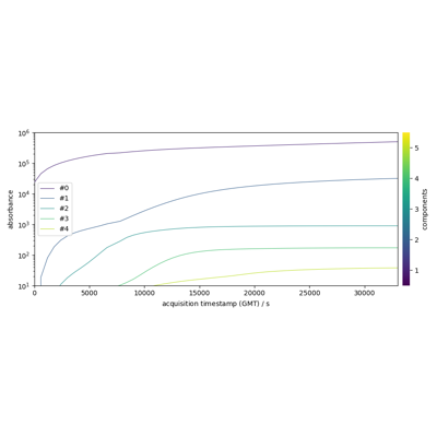
plot_score(scores=None, components=(1, 2), **kwargs)[source]

2D or 3D score plot of observations.

Plots the projection of each observation/spectrum onto the span of two or three selected principal components.

Parameters:

scores (NDDataset or tuple, optional) – Scores dataset to plot. If None, uses self.scores. Pass a modified scores dataset (e.g., with custom labels) to use those labels in the plot.

Note: If a tuple or list is passed as the first positional argument, it is interpreted as components for backward compatibility.
components (tuple of int, optional) – Principal components to plot (1-based indexing). Length 2 for 2D plot, length 3 for 3D plot. Default: (1, 2).
**kwargs – Additional keyword arguments passed to plot_score. See plot_score for available options:
- cmap : Colormap for coloring points.
- color : Fixed color or color values for each point.
- color_mapping : “index” (default) or “labels” - how to map colors.
- show_labels : If True, annotate points with labels.
- labels_column : Column index in scores.y.labels (0-based).
- ax : Axes to plot on.
- show : Whether to display the figure.

Returns:

matplotlib.axes.Axes – The matplotlib axes.

See also

plot_score: Standalone score plot function.

Examples

>>> import spectrochempy as scp
>>> X = scp.read("irdata/nh4y-activation.spg")
>>> pca = scp.PCA(n_components=5)
>>> pca.fit(X)
>>> ax = pca.plot_score((1, 2), show=False)  

With custom labels:

>>> scores = pca.transform()  
>>> scores.y.labels = custom_labels  
>>> ax = pca.plot_score(scores=scores, show_labels=True)  

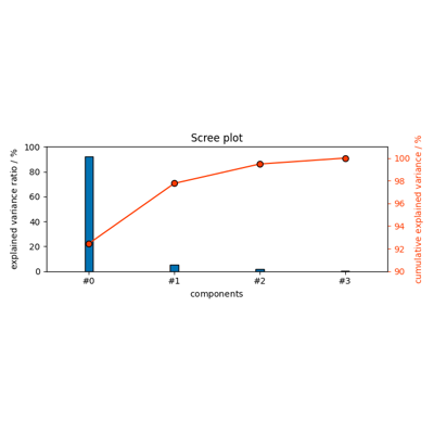
plot_scree(n_components=None, **kwargs)[source]

Scree plot of explained variance + cumulative variance by PCA.

Explained variance by each PC is plotted as a bar graph (left y axis) and cumulative explained variance is plotted as a line with markers (right y axis).

Parameters:

n_components (int, optional) – Number of components to plot. If None, plots all components.
**kwargs – Additional keyword arguments passed to plot_scree. See plot_scree for available options (e.g., bar_color, line_color, title, ax, show).

Returns:

matplotlib.axes.Axes – The primary axes (left y-axis with bars).

See also

plot_scree: Standalone scree plot function.

Examples

>>> import spectrochempy as scp
>>> X = scp.read("irdata/nh4y-activation.spg")
>>> pca = scp.PCA(n_components=5)
>>> pca.fit(X)
>>> ax = pca.plot_scree(show=False)  

plotmerit(X=None, X_hat=None, **kwargs)[source]

Plot the input (X), reconstructed (X_hat) and residuals.

\(X\) and \(\hat{X}\) can be passed as arguments. If not, the X attribute is used for \(X`and :math:\)hat{X}`is computed by the inverse_transform method

Parameters:

X (NDDataset, optional) – Original dataset. If is not provided (default), the X attribute is used and X_hat is computed using inverse_transform.
X_hat (NDDataset, optional) – Inverse transformed dataset. if X is provided, X_hat must also be provided as compuyed externally.

Returns:

Axes – Matplotlib subplot axe.

Other Parameters:

exp_c (color, colormap, or list of colors, optional) – Color(s) for experimental spectra. - None: use unified semantic resolver (auto-detect categorical/sequential) - Single color: use for all experimental spectra - Colormap name/object: sample colors from colormap - List/tuple: use as explicit color cycle
calc_c (color, colormap, or list of colors, optional) – Color(s) for calculated spectra. - None: use default blue “#2a6fbb” - Single color: use for all calculated spectra - Colormap name/object: sample colors from colormap - List/tuple: use as explicit color cycle
resid_c (color, colormap, or list of colors, optional) – Color(s) for residual spectra. - None: use default grey “0.4” - Single color: use for all residual spectra - Colormap name/object: sample colors from colormap - List/tuple: use as explicit color cycle
exp_linestyle (str, optional) – Line style for experimental spectra. Default: “-“.
calc_linestyle (str, optional) – Line style for calculated spectra. Default: “–“.
resid_linestyle (str, optional) – Line style for residual spectra. Default: “-“.
exp_linewidth (float, optional) – Line width for experimental spectra. Default: 1.2.
calc_linewidth (float, optional) – Line width for calculated spectra. Default: 1.0.
resid_linewidth (float, optional) – Line width for residual spectra. Default: 1.0.
min_contrast (float, optional) – Minimum contrast ratio for sequential colormaps. Default: 1.5.
offset (float, optional, default: None) – Specify the separation (in percent) between the \(X\) , \(X_hat\) and \(E\).
nb_traces (int or 'all', optional) – Number of lines to display. Default is 'all'.
**others (Other keywords parameters) – Parameters passed to the internal plot method of the X dataset.

printev(n_components=None)[source]

Print PCA figures of merit.

Prints eigenvalues and explained variance for all or first n_pc PC’s.

Parameters:: n_components (int, optional) – The number of components to print.

reconstruct(X_transform=None, **kwargs)[source]

Transform data back to its original space.

In other words, return an input X_original whose reduce/transform would be X_transform.

Parameters:

X_transform (array-like of shape (n_observations, n_components), optional) – Reduced X data, where n_observations is the number of observations and n_components is the number of components. If X_transform is not provided, a transform of X provided in fit is performed first.
**kwargs (keyword parameters, optional) – See Other Parameters.

Returns:

NDDataset – Dataset with shape (n_observations, n_features).

Other Parameters:

n_components (int, optional) – The number of components to use for the reduction. If not given the number of components is eventually the one specified or determined in the fit process.

See also

reconstruct: Alias of inverse_transform (Deprecated).

Notes

Deprecated in version 0.6.

reduce(X=None, **kwargs)[source]

Apply dimensionality reduction to X.

Parameters:

X (NDDataset or array-like of shape (n_observations, n_features), optional) – New data, where n_observations is the number of observations and n_features is the number of features. if not provided, the input dataset of the fit method will be used.
**kwargs (keyword parameters, optional) – See Other Parameters.

Returns:

NDDataset – Dataset with shape (n_observations, n_components).

Other Parameters:

n_components (int, optional) – The number of components to use for the reduction. If not given the number of components is eventually the one specified or determined in the fit process.

Notes

Deprecated in version 0.6.

reset()[source]: Reset configuration parameters to their default values.

scoreplot(self, *args, **kwargs)[source]

2D or 3D scoreplot of observations.

Deprecated since version 0.7.4: Use plot_score instead.

Parameters:

*args – Positional arguments. Accepts: - (i, j) or (i, j, k): component indices (1-based) - (scores, i, j): NDDataset and component indices
**kwargs – Additional keyword arguments passed to plot_score.

Returns:

matplotlib.axes.Axes – The matplotlib axes.

screeplot(n_components=None, **kwargs)[source]

Scree plot of explained variance + cumulative variance by PCA.

Deprecated since version 0.7.4: Use plot_scree instead.

Parameters:

n_components (int, optional) – Number of components to plot.
**kwargs – Additional keyword arguments (ignored, for backward compatibility).

Returns:

matplotlib.axes.Axes – The primary axes.

to_dict()[source]

Return config value in a dict form.

Returns:: dict – A regular dictionary.

transform(X=None, **kwargs)

Apply dimensionality reduction to X.

Parameters:

X (NDDataset or array-like of shape (n_observations, n_features), optional) – New data, where n_observations is the number of observations and n_features is the number of features. if not provided, the input dataset of the fit method will be used.
**kwargs (keyword parameters, optional) – See Other Parameters.

Returns:

NDDataset – Dataset with shape (n_observations, n_components).

Other Parameters:

n_components (int, optional) – The number of components to use for the reduction. If not given the number of components is eventually the one specified or determined in the fit process.

Examples using spectrochempy.PCA

EFA example

PCA example (iris dataset)

PCA analysis example